Process and observation uncertainty explained with R

Once upon a time I had grand ambitions of writing blog posts outlining all of the examples in the Ecological Detective.¹ A few years ago I participated in a graduate seminar series where we went through many of the examples in this book. I am not a population biologist by trade but many of the concepts were useful for not only helping me better understand core concepts of statistical modelling, but also for developing an appreciation of the limits of your data. Part of this appreciation stems from understanding sources and causes of uncertainty in estimates. Perhaps in the future I will focus more blog topics on other examples from The Ecological Detective, but for now I’d like to discuss an example that has recently been of interest in my own research.

Over the past few months I have been working with some colleagues to evaluate statistical power of biological indicators. These analyses are meant to describe the certainty within which a given level of change in an indicator is expected over a period of time. For example, what is the likelihood of detecting a 50% decline over twenty years considering that our estimate of the indicators are influenced by uncertainty? We need reliable estimates of the uncertainty to answer these types of questions and it is often useful to categorize sources of variation. Hilborn and Mangel describe process and observation uncertainty as two primary categories of noise in a data measurement. Process uncertainty describes noise related to actual or real variation in a measurement that a model does not describe. For example, a model might describe response of an indicator to changing pollutant loads but we lack an idea of seasonal variation that occurs naturally over time. Observation uncertainty is often called sampling uncertainty and describes our ability to obtain a precise data measurement. This is a common source of uncertainty in ecological data where precision of repeated surveys may be affected by several factors, such as skill level of the field crew, precision of sampling devices, and location of survey points. The effects of process and observation uncertainty on data measurements are additive such that the magnitude of both can be separately estimated.

The example I’ll focus on is described on pages 59–61 (the theory) and 90–92 (an example with pseudocode) in The Ecological Detective. This example describes an approach for conceptualizing the effects of uncertainty on model estimates, as opposed to methods for quantifying uncertainty from actual data. For the most part, this blog is an exact replica of the example, although I have tried to include some additional explanation where I had difficulty understanding some of the concepts. Of course, I’ll also include R code since that’s the primary motivation for my blog.

We start with a basic population model that describes population change over time. This is a theoretical model that, in practice, should describe some actual population, but is very simple for the purpose of learning about sources of uncertainty. From this basic model, we simulate sources of uncertainty to get an idea of their exact influence on our data measurements. The basic model without imposing uncertainty is as follows:

where the population at time is equal to the population at time multiplied by the survival probability plus the number of births at time . We call this the process model because it’s meant to describe an actual population process, i.e., population growth over time given birth and survival. We can easily create a function to model this process over a time series. As in the book example, we’ll use a starting population of fifty individuals, add 20 individuals from births at each time step, and use an 80% survival rate.

# simple pop model
proc_mod <- function(N_0 = 50, b = 20, s = 0.8, t = 50){
	
	N_out <- numeric(length = t)
	N_out[1] <- N_0
	
	for(step in 1:t) 
		N_out[step + 1] <- s*N_out[step] + b
	
	out <- data.frame(steps = 1:t, Pop = N_out[-1])
	
	return(out)
	
}

est <- proc_mod()

The model is pretty straightforward. A for loop is used to estimate the population for time steps one to fifty with a starting population size of fifty at time zero. Each time step multiplies the population estimate from the previous time step and adds twenty new individuals. You may notice that the function could easily be vectorized, but I’ve used a for loop to account for sources of uncertainty that are dependent on previous values in the time series. This will be explained below but for now the model only describes the actual process.

The results are assigned to the est object and then plotted.

library(ggplot2)
ggplot(est, aes(steps, Pop)) + 
	geom_point() + 
	theme_bw() + 
	ggtitle('N_0 = 50, s = 0.8, b = 20\n')

Fig: Population over time using a simplified process model.

In a world with absolute certainty, an actual population would follow this trend if our model accurately described the birth and survivorship rates. Suppose our model provided an incomplete description of the population. Hilborn and Mangel (p. 59) suggest that birth rates, for example, may fluctuate from year to year. This fluctuation is not captured by our model and represents a source of process uncertainty, or uncertainty caused by an incomplete description of the process. We can assume that the effect of this process uncertainty is additive to the population estimate at each time step:

where the model remains the same but we’ve included an additional term, , to account for uncertainty. This uncertainty is random in the sense that we don’t know exactly how it will influence our estimate but we can describe it as a random variable from a known distribution. Suppose we expect random variation in birth rates for each time step to be normally distributed with mean zero and a given standard deviation. Population size at is the survivorship of the population at time plus the births accounting for random variation. An important point is that the random variation is additive throughout the time series. That is, if more births were observed for a given year due to random chance, the population would be larger the next year such that additional random variation at is added to the larger population. This is why a for loop is used because we can’t simulate uncertainty by adding a random vector all at once to the population estimates.

The original model is modified to include process uncertainty.

# simple pop model with process uncertainty 
proc_mod2 <- function(N_0 = 50, b = 20, s = 0.8, t = 50, 
        sig_w = 5){
	
	N_out <- numeric(length = t + 1)
	N_out[1] <- N_0
	
	sig_w <- rnorm(t, 0, sig_w)
	
	for(step in 1:t) 
		N_out[step + 1] <- s*N_out[step] + b + sig_w[step]
	
	out <- data.frame(steps = 1:t, Pop = N_out[-1])
	
	return(out)
	
}

set.seed(2)
est2 <- proc_mod2()

# plot the estimates
ggt <- paste0('N_0 = 50, s = 0.8, b = 20, sig_w = ',formals(proc_mod)$sig_w,'\n')
ggplot(est2, aes(steps, Pop)) + 
	geom_point() + 
	theme_bw() + 
	ggtitle(ggt)

Fig: Population over time using a simplified process model that includes process uncertainty.

We see considerable variation from the original model now that we’ve included process uncertainty. Note that the process uncertainty in each estimate is dependent on the estimate prior, as described above. This creates uncertainty that, although random, follows a pattern throughout the time series. We can look at an auto-correlation plot of the new estimates minus the actual population values to get an idea of this pattern. Observations that are closer to one another in the time series are correlated, as expected.

Fig: Auto-correlation between observations with process uncertainty at different time lags.

Adding observation uncertainty is simpler in that the effect is not propagated throughout the time steps. Rather, the uncertainty is added after the time series is generated. This makes intuitive because the observation uncertainty describes sampling error. For example, if we have an instrument malfunction one year that creates an unreliable estimate we can fix the instrument to get a more accurate reading the next year. However, suppose we have a new field crew the following year that contributes to uncertainty (e.g., wrong species identification). This uncertainty is not related to the year prior. Computationally, the model is as follows:

where the model is identical to the deterministic model with the addition of observation uncertainty after the time series is calculated for fifty time steps. is the population estimate for the whole time series and is the estimate including observation uncertainty. We can simulate observation uncertainty using a random normal variable with assumed standard deviation as we did with process uncertainty, e.g., has length fifty with mean zero and standard deviation equal to five.

# model with observation uncertainty
proc_mod3 <- function(N_0 = 50, b = 20, s = 0.8, t = 50, sig_v = 5){
	
	N_out <- numeric(length = t)
	N_out[1] <- N_0
	
	sig_v <- rnorm(t, 0, sig_v)
	
	for(step in 1:t) 
		N_out[step + 1] <- s*N_out[step] + b
	
	N_out <- N_out + c(NA,sig_v)
	
	out <- data.frame(steps = 1:t, Pop = N_out[-1])
	
	return(out)
	
}

# get estimates
set.seed(3)
est3 <- proc_mod3()

# plot
ggt <- paste0('N_0 = 50, s = 0.8, b = 20, sig_v = ',
        formals(proc_mod3)$sig_v,'\n')
ggplot(est3, aes(steps, Pop)) + 
        geom_point() + 
	theme_bw() + 
	ggtitle(ggt)

Fig: Population over time using a simplified process model that includes observation uncertainty.

We can confirm that the observations are not correlated between the time steps, unlike the model with process uncertainty.

Fig: Auto-correlation between observations with observation uncertainty at different time lags.

Now we can create a model that includes both process and observation uncertainty by combining the above functions. The function is slightly tweaked to return include a data frame with all estimates: process model only, process model with process uncertainty, process model with observation uncertainty, process model with process and observation uncertainty.

# combined function
proc_mod_all <- function(N_0 = 50, b = 20, s = 0.8, t = 50, 
        sig_w = 5, sig_v = 5){
	
	N_out <- matrix(NA, ncol = 4, nrow = t + 1)
	N_out[1,] <- N_0
	
	sig_w <- rnorm(t, 0, sig_w)
	sig_v <- rnorm(t, 0, sig_v)
	
	for(step in 1:t){
		N_out[step + 1, 1] <- s*N_out[step] + b
		N_out[step + 1, 2] <- N_out[step, 1] + sig_w[step]
		}
	
	N_out[1:t + 1, 3]  <- N_out[1:t + 1, 1] + sig_v
		
	N_out[1:t + 1, 4]  <- N_out[1:t + 1, 2] + sig_v
	
	out <- data.frame(1:t,N_out[-1,])
	names(out) <- c('steps', 'mod_act', 'mod_proc', 'mod_obs', 'mod_all')
	
	return(out)
	
}

# create data
set.seed(2)
est_all <- proc_mod_all()

# plot the data
library(reshape2)
to_plo <- melt(est_all, id.var = 'steps')

# re-assign factor labels for plotting
to_plo$variable <- factor(to_plo$variable, levels = levels(to_plo$variable),
	labels = c('Actual','Pro','Obs','Pro + Obs'))

ggplot(to_plo, aes(steps, value)) + 
	geom_point() + 
	facet_wrap(~variable) + 
	ylab('Pop. estimate') + 
	theme_bw()

Fig: Population over time using a simplified process model that includes no uncertainty (actual), process uncertainty (Pro), observation uncertainty (Obs), and both (Pro + Obs).

On the surface, the separate effects of process and observation uncertainty on the estimates is similar, whereas the effects of adding both maximizes the overall uncertainty. We can quantify the extent to which the sources of uncertainty influence the estimates by comparing observations at time to observations at . In other words, we can quantify the variance for each model by regressing observations separated by one time lag. We would expect the model that includes both sources of uncertainty to have the highest variance.

# comparison of mods
# create vectors for pop estimates at time t (t_1) and t - 1 (t_0)
t_1 <- est_all[2:nrow(est_all),-1]
t_1 <- melt(t_1, value.name = 'val_1')
t_0 <- est_all[1:(nrow(est_all)-1),-1]
t_0 <- melt(t_0, value.name = 'val_0')

#combine for plotting
to_plo2 <- cbind(t_0,t_1[,!names(t_1) %in% 'variable',drop = F])
head(to_plo2)
##   variable   val_0    val_1
## 1  mod_act 60.0000 68.00000
## 2  mod_act 68.0000 74.40000
## 3  mod_act 74.4000 79.52000
## 4  mod_act 79.5200 83.61600
## 5  mod_act 83.6160 86.89280
## 6  mod_act 86.8928 89.51424

# re-assign factor labels for plotting
to_plo2$variable <- factor(to_plo2$variable, levels = levels(to_plo2$variable),
	labels = c('Actual','Pro','Obs','Pro + Obs'))

# we don't want to plot the first process model
sub_dat <- to_plo2$variable == 'Actual'
ggplot(to_plo2[!sub_dat,], aes(val_0, val_1)) + 
	geom_point() + 
	facet_wrap(~variable) + 
	theme_bw() + 
	scale_y_continuous('Population size at time t') + 
	scale_x_continuous('Population size at time t - 1') +
	geom_abline(slope = 0.8, intercept = 20)

Fig: Evaluation of uncertainty in population estimates affected by process uncertainty (Pro), observation uncertainty (Obs), and both (Pro + Obs). The line indicates data from the actual process model without uncertainty.

A tabular comparison of the regressions for each plot provides a quantitative measure of the effect of uncertainty on the model estimates.

library(stargazer)
mods <- lapply(
	split(to_plo2,to_plo2$variable), 
	function(x) lm(val_1~val_0, data = x)
	)
stargazer(mods, omit.stat = 'f', title = 'Regression of population estimates at time $t$ against time $t - 1$ for each process model.  Each model except the first simulates different sources of uncertainty.', column.labels = c('Actual','Pro','Obs','Pro + Obs'), model.numbers = F)

The table tells us exactly what we would expect. Based on the r-squared values, adding more uncertainty decreases the explained variance of the models. Also note the changes in the parameter estimates. The actual model provides slope and intercept estimates identical to those we specified in the beginning ( and ). Adding more uncertainty to each model contributes to uncertainty in the parameter estimates such that survivorship is under-estimated and birth contributions are over-estimated.

It’s nice to use an arbitrary model where we can simulate effects of uncertainty, unlike situations with actual data where sources of uncertainty are not readily apparent. This example from The Ecological Detective is useful for appreciating the effects of uncertainty on parameter estimates in simple process models. I refer the reader to the actual text for more discussion regarding the implications of these analyses. Also, check out Ben Bolker’s text² (chapter 11) for more discussion with R examples.

Cheers,

Marcus

¹Hilborn R, Mangel M. 1997. The Ecological Detective: Confronting Models With Data. Monographs in Population Biology 28. Princeton University Press. Princeton, New Jersey. 315 pages.
²Bolker B. 2007. Ecological Models and Data in R. Princeton University Press. Princeton, New Jersey. 508 pages.

Brief introduction on Sweave and Knitr for reproducible research

A few weeks ago I gave a presentation on using Sweave and Knitr under the guise of promoting reproducible research. I humbly offer this presentation to the blog with full knowledge that there are already loads of tutorials available online. This presentation is specific and slightly biased towards Windows OS, so it probably has limited relevance if you are interested in other methods. Anyhow, I hope this is useful to some of you.

Cheers,

Marcus

\documentclass[xcolor=svgnames]{beamer}
%\documentclass[xcolor=svgnames,handout]{beamer}
\usetheme{Boadilla}
\usecolortheme[named=Sienna]{structure}
\usepackage{graphicx}
\usepackage[final]{animate}
%\usepackage[colorlinks=true,urlcolor=blue,citecolor=blue,linkcolor=blue]{hyperref}
\usepackage{breqn}
\usepackage{xcolor}
\usepackage{booktabs}
\usepackage{verbatim}
\usepackage{tikz}
\usetikzlibrary{shadows,arrows,positioning}
\usepackage[noae]{Sweave}
\definecolor{links}{HTML}{2A1B81}
\hypersetup{colorlinks,linkcolor=links,urlcolor=links}
\usepackage{pgfpages}
%\pgfpagesuselayout{4 on 1}[letterpaper, border shrink = 5mm, landscape]

\tikzstyle{block} = [rectangle, draw, text width=7em, text centered, rounded corners, minimum height=3em, minimum width=7em, top color = white, bottom color=brown!30,  drop shadow]

\newcommand{\ShowSexpr}[1]{\texttt{{\char`\\}Sexpr\{#1\}}}

\begin{document}
\SweaveOpts{concordance=TRUE}

\title[Nuts and bolts of Sweave/Knitr]{The nuts and bolts of Sweave/Knitr for reproducible research with \LaTeX}
\author[M. Beck]{Marcus W. Beck}

\institute[USEPA NHEERL]{ORISE Post-doc Fellow\\
USEPA NHEERL Gulf Ecology Division, Gulf Breeze, FL\\
Email: \href{mailto:beck.marcus@epa.gov}{beck.marcus@epa.gov}, Phone: 850 934 2480}

\date{January 15, 2014}

%%%%%%
\begin{frame}
\vspace{-0.3in}
\titlepage
\end{frame}

%%%%%%
\begin{frame}{Reproducible research}
\onslide<+->
In it's most general sense... the ability to reproduce results from an experiment or analysis conducted by another.\\~\\
\onslide<+->
From Wikipedia... `The ultimate product is the \alert{paper along with the full computational environment} used to produce the results in the paper such as the code, data, etc. that can be \alert{used to reproduce the results and create new work} based on the research.'\\~\\
\onslide<+->
Concept is strongly based on the idea of \alert{literate programming} such that the logic of the analysis is clearly represented in the final product by combining computer code/programs with ordinary human language [Knuth, 1992].
\end{frame}

%%%%%%
\begin{frame}{Non-reproducible research}
\begin{center}
\begin{tikzpicture}[node distance=2.5cm, auto, >=stealth]
	\onslide<2->{
	\node[block] (a) {1. Gather data};}
	\onslide<3->{
	\node[block] (b)  [right of=a, node distance=4.2cm] {2. Analyze data};
 	\draw[->] (a) -- (b);}
 	\onslide<4->{
 	\node[block] (c)  [right of=b, node distance=4.2cm]  {3. Report results};
 	\draw[->] (b) -- (c);}
%  	\onslide<5->{
%  	\node [right of=a, node distance=2.1cm] {\textcolor[rgb]{1,0,0}{X}};
%  	\node [right of=b, node distance=2.1cm] {\textcolor[rgb]{1,0,0}{X}};}
\end{tikzpicture}
\end{center}
\vspace{-0.5cm}
\begin{columns}[t]
\onslide<2->{
\begin{column}{0.33\textwidth}
\begin{itemize}
\item Begins with general question or research objectives
\item Data collected in raw format (hard copy) converted to digital (Excel spreadsheet)
\end{itemize}
\end{column}}
\onslide<3->{
\begin{column}{0.33\textwidth}
\begin{itemize}
\item Import data into stats program or analyze directly in Excel
\item Create figures/tables directly in stats program
\item Save relevant output
\end{itemize}
\end{column}}
\onslide<4->{
\begin{column}{0.33\textwidth}
\begin{itemize}
\item Create research report using Word or other software
\item Manually insert results into report
\item Change final report by hand if methods/analysis altered
\end{itemize}
\end{column}}
\end{columns}

\end{frame}

%%%%%%
\begin{frame}{Reproducible research}
\begin{center}
\begin{tikzpicture}[node distance=2.5cm, auto, >=stealth]
	\onslide<1->{
	\node[block] (a) {1. Gather data};}
	\onslide<1->{
	\node[block] (b)  [right of=a, node distance=4.2cm] {2. Analyze data};
 	\draw[<->] (a) -- (b);}
 	\onslide<1->{
 	\node[block] (c)  [right of=b, node distance=4.2cm]  {3. Report results};
 	\draw[<->] (b) -- (c);}
\end{tikzpicture}
\end{center}
\vspace{-0.5cm}
\begin{columns}[t]
\onslide<1->{
\begin{column}{0.33\textwidth}
\begin{itemize}
\item Begins with general question or research objectives
\item Data collected in raw format (hard copy) converted to digital (\alert{text file})
\end{itemize}
\end{column}}
\onslide<1->{
\begin{column}{0.33\textwidth}
\begin{itemize}
\item Create \alert{integrated script} for importing data (data path is known) 
\item Create figures/tables directly in stats program
\item \alert{No need to export} (reproduced on the fly)
\end{itemize}
\end{column}}
\onslide<1->{
\begin{column}{0.33\textwidth}
\begin{itemize}
\item Create research report using RR software
\item \alert{Automatically include results} into report
\item \alert{Change final report automatically} if methods/analysis altered
\end{itemize}
\end{column}}
\end{columns}

\end{frame}

%%%%%%
\begin{frame}{Reproducible research in R}
Easily adopted using RStudio [\href{http://www.rstudio.com/}{http://www.rstudio.com/}]\\~\\
Also possible w/ Tinn-R or via command prompt but not as intuitive\\~\\
Requires a \LaTeX\ distribution system - use MikTex for Windows [\href{http://miktex.org/}{http://miktex.org/}]\\~\\
\onslide<2->{
Essentially a \LaTeX\ document that incorporates R code... \\~\\
Uses Sweave (or Knitr) to convert .Rnw file to .tex file, then \LaTeX\ to create pdf\\~\\
Sweave comes with \texttt{utils} package, may have to tell R where it is \\~\\
}
\end{frame}

%%%%%%
\begin{frame}{Reproducible research in R}
Use same procedure for compiling a \LaTeX\ document with one additional step

\begin{center}
\begin{tikzpicture}[node distance=2.5cm, auto, >=stealth]
	\onslide<2->{
	\node[block] (a) {1. myfile.Rnw};}
	\onslide<3->{
	\node[block] (b)  [right of=a, node distance=4.2cm] {2. myfile.tex};
 	\draw[->] (a) -- (b);\node [right of=a, above=0.5cm, node distance=2.1cm] {Sweave};}
 	\onslide<4->{
 	\node[block] (c)  [right of=b, node distance=4.2cm]  {3. myfile.pdf};
 	\draw[->] (b) -- (c);
 	\node [right of=b, above=0.5cm, node distance=2.1cm] {pdfLatex};}
\end{tikzpicture}
\end{center}
\vspace{-0.5cm}
\begin{columns}[t]
\onslide<2->{
\begin{column}{0.33\textwidth}
\begin{itemize}
\item A .tex file but with .Rnw extension
\item Includes R code as `chunks' or inline expressions
\end{itemize}
\end{column}}
\onslide<3->{
\begin{column}{0.33\textwidth}
\begin{itemize}
\item .Rnw file is converted to a .tex file using Sweave
\item .tex file contains output from R, no raw R code
\end{itemize}
\end{column}}
\onslide<4->{
\begin{column}{0.33\textwidth}
\begin{itemize}
\item .tex file converted to pdf (or other output) for final format
\item Include biblio with bibtex
\end{itemize}
\end{column}}
\end{columns}

\end{frame}

%%%%%%
\begin{frame}[containsverbatim]{Reproducible research in R} \label{sweaveref}
\begin{block}{.Rnw file}
\begin{verbatim}
\documentclass{article}
\usepackage{Sweave}

\begin{document}

Here's some R code:

\Sexpr{'<<eval=true,echo=true>>='}
options(width=60)
set.seed(2)
rnorm(10)
\Sexpr{'@'}

\end{document}
\end{verbatim}
\end{block}

\end{frame}

%%%%%%
\begin{frame}[containsverbatim,shrink]{Reproducible research in R}
\begin{block}{.tex file}
\begin{verbatim}
\documentclass{article}
\usepackage{Sweave}

\begin{document}

Here's some R code:

\begin{Schunk}
\begin{Sinput}
> options(width=60)
> set.seed(2)
> rnorm(10)
\end{Sinput}
\begin{Soutput}
 [1] -0.89691455  0.18484918  1.58784533 -1.13037567  
 [5] -0.08025176  0.13242028  0.70795473 -0.23969802  
 [9]  1.98447394 -0.13878701
\end{Soutput}
\end{Schunk}

\end{document}
\end{verbatim}
\end{block}

\end{frame}

%%%%%%
\begin{frame}{Reproducible research in R}
The final product:\\~\\
\centerline{\includegraphics{ex1_input.pdf}}
\end{frame}

%%%%%%
\begin{frame}[fragile]{Sweave - code chunks}
\onslide<+->
R code is entered in the \LaTeX\ document using `code chunks'
\begin{block}{}
\begin{verbatim}
\Sexpr{'<<>>='}
\Sexpr{'@'}
\end{verbatim}
\end{block}
Any text within the code chunk is interpreted as R code\\~\\
Arguments for the code chunk are entered within \verb|\Sexpr{'<<here>>'}|\\~\\
\onslide<+->
\begin{itemize}
\item{\texttt{eval}: evaluate code, default \texttt{T}}
\item{\texttt{echo}: return source code, default \texttt{T}}
\item{\texttt{results}: format of output (chr string), default is `include' (also `tex' for tables or `hide' to suppress)}
\item{\texttt{fig}: for creating figures, default \texttt{F}}
\end{itemize}
\end{frame}

%%%%%%
\begin{frame}[fragile]{Sweave - code chunks}
Changing the default arguments for the code chunk:
\begin{columns}[t]
\begin{column}{0.45\textwidth}
\onslide<+->
\begin{block}{}
\begin{verbatim}
\Sexpr{'<<>>='}
2+2
\Sexpr{'@'}
\end{verbatim}
\end{block}
<<>>=
2+2
@
\onslide<+->
\begin{block}{}
\begin{verbatim}
\Sexpr{'<<eval=F,echo=F>>='}
2+2
\Sexpr{'@'}
\end{verbatim}
\end{block}
Returns nothing...
\end{column}
\begin{column}{0.45\textwidth}
\onslide<+->
\begin{block}{}
\begin{verbatim}
\Sexpr{'<<eval=F>>='}
2+2
\Sexpr{'@'}
\end{verbatim}
\end{block}
<<eval=F>>=
2+2
@
\onslide<+->
\begin{block}{}
\begin{verbatim}
\Sexpr{'<<echo=F>>='}
2+2
\Sexpr{'@'}
\end{verbatim}
\end{block}
<<echo=F>>=
2+2
@
\end{column}
\end{columns}
\end{frame}

%%%%%%
\begin{frame}[t,fragile]{Sweave - figures}
\onslide<1->
Sweave makes it easy to include figures in your document
\begin{block}{}
\begin{verbatim}
\Sexpr{'<<myfig,fig=T,echo=F,include=T,height=3>>='}
set.seed(2)
hist(rnorm(100))
\Sexpr{'@'}
\end{verbatim}
\end{block}
\onslide<2->
<<myfig,fig=T,echo=F,include=T,height=3>>=
set.seed(2)
hist(rnorm(100))
@
\end{frame}

%%%%%%
\begin{frame}[t,fragile]{Sweave - figures}
Sweave makes it easy to include figures in your document
\begin{block}{}
\begin{verbatim}
\Sexpr{'<<myfig,fig=T,echo=F,include=T,height=3>>='}
set.seed(2)
hist(rnorm(100))
\Sexpr{'@'}
\end{verbatim}
\end{block}
\vspace{\baselineskip}
Relevant code options for figures:
\begin{itemize}
\item{The chunk name is used to name the figure, myfile-myfig.pdf}
\item{\texttt{fig}: Lets R know the output is a figure}
\item{\texttt{echo}: Use \texttt{F} to suppress figure code}
\item{\texttt{include}: Should the figure be automatically include in output}
\item{\texttt{height}: (and \texttt{width}) Set dimensions of figure in inches}
\end{itemize}
\end{frame}

%%%%%%
\begin{frame}[t,fragile]{Sweave - figures}
An alternative approach for creating a figure
\begin{block}{}
\begin{verbatim}
\Sexpr{'<<myfig,fig=T,echo=F,include=F,height=3>>='}
set.seed(2)
hist(rnorm(100))
\Sexpr{'@'}
\includegraphics{rnw_name-myfig.pdf}
\end{verbatim}
\end{block}
\includegraphics{Sweave_intro-myfig.pdf}
\end{frame}

%%%%%%
\begin{frame}[t,fragile]{Sweave - tables}
\onslide<1->
Really easy to create tables
\begin{block}{}
\begin{verbatim}
\Sexpr{'<<results=tex,echo=F>>='}
library(stargazer)
data(iris)
stargazer(iris,title='Summary statistics for Iris data')
\Sexpr{'@'}
\end{verbatim}
\end{block}
\onslide<2->
<<results=tex,echo=F>>=
data(iris)
library(stargazer)
stargazer(iris,title='Summary statistics for Iris data')
@

\end{frame}

%%%%%%
\begin{frame}[t,fragile]{Sweave - tables}
Really easy to create tables
\begin{block}{}
\begin{verbatim}
\Sexpr{'<<results=tex,echo=F>>='}
library(stargazer)
data(iris)
stargazer(iris,title='Summary statistics for Iris data')
\Sexpr{'@'}
\end{verbatim}
\end{block}
\vspace{\baselineskip}
\texttt{results} option should be set to `tex' (and \texttt{echo=F})\\~\\
Several packages are available to convert R output to \LaTeX\ table format
\begin{itemize}
\item{xtable: most general package}
\item{hmisc: similar to xtable but can handle specific R model objects}
\item{stargazer: fairly effortless conversion of R model objects to tables}
\end{itemize}
\end{frame}

%%%%%%
\begin{frame}[fragile]{Sweave - expressions}
\onslide<1->
All objects within a code chunk are saved in the workspace each time a document is compiled (unless \texttt{eval=F})\\~\\
This allows the information saved in the workspace to be reproduced in the final document as inline text, via \alert{expressions}\\~\\
\onslide<2->
\begin{block}{}
\begin{verbatim}
\Sexpr{'<<echo=F>>='}
data(iris)
dat<-iris
\Sexpr{'@'}
\end{verbatim}
Mean sepal length was \ShowSexpr{mean(dat\$Sepal.Length)}.
\end{block}
\onslide<3->
<<echo=F>>=
data(iris)
dat<-iris
@
\vspace{\baselineskip}
Mean sepal length was \Sexpr{mean(dat$Sepal.Length)}.
\end{frame}

%%%%%%
\begin{frame}[fragile]{Sweave - expressions}
Change the global R options to change the default output\\~\\
\begin{block}{}
\begin{verbatim}
\Sexpr{'<<echo=F>>='}
data(iris)
dat<-iris
options(digits=2)
\Sexpr{'@'}
\end{verbatim}
Mean sepal length was \ShowSexpr{format(mean(dat\$Sepal.Length))}.
\end{block}
<<echo=F>>=
data(iris)
dat<-iris
options(digits=2)
@
\vspace{\baselineskip}
Mean sepal length was \Sexpr{format(mean(dat$Sepal.Length))}.\\~\\
\end{frame}

%%%%%%
\begin{frame}{Sweave vs Knitr}
\onslide<1->
Does not automatically cache R data on compilation\\~\\
\alert{Knitr} is a useful alternative - similar to Sweave but with minor differences in args for code chunks, more flexible output\\~\\
\onslide<2->
\begin{columns}
\begin{column}{0.3\textwidth}
Must change default options in RStudio\\~\\
Knitr included with RStudio, otherwise download as package
\end{column}
\begin{column}{0.6\textwidth}
\centerline{\includegraphics[width=0.8\textwidth]{options_ex.png}}
\end{column}
\end{columns}
\end{frame}

%%%%%%
\begin{frame}[fragile]{Knitr}
\onslide<1->
Knitr can be used to cache code chunks\\~\\
Date are saved when chunk is first evaluated, skipped on future compilations unless changed\\~\\
This allows quicker compilation of documents that import lots of data\\
~\\
\begin{block}{}
\begin{verbatim}
\Sexpr{'<<mychunk, cache=TRUE, eval=FALSE>>='}
load(file='mydata.RData')
\Sexpr{'@'}
\end{verbatim}
\end{block}
\end{frame}

%%%%%%
\begin{frame}[containsverbatim,shrink]{Knitr} \label{knitref}
\begin{block}{.Rnw file}
\begin{verbatim}
\documentclass{article}

\Sexpr{'<<setup, include=FALSE, cache=FALSE>>='}
library(knitr)

#set global chunk options
opts_chunk$set(fig.path='H:/docs/figs/', fig.align='center', 
dev='pdf', dev.args=list(family='serif'), fig.pos='!ht')

options(width=60)
\Sexpr{'@'}

\begin{document}

Here's some R code:

\Sexpr{'<<eval=T, echo=T>>='}
set.seed(2)
rnorm(10)
\Sexpr{'@'}

\end{document}
\end{verbatim}
\end{block}

\end{frame}

%%%%%%
\begin{frame}{Knitr}
The final product:\\~\\
\centerline{\includegraphics[width=\textwidth]{knit_ex.pdf}}
\end{frame}

%%%%%%
\begin{frame}[containsverbatim,shrink]{Knitr}
Figures, tables, and expressions are largely the same as in Sweave\\~\\

\begin{block}{Figures}
\begin{verbatim}
\Sexpr{'<<myfig,echo=F>>='}
set.seed(2)
hist(rnorm(100))
\Sexpr{'@'}
\end{verbatim}
\end{block}
\vspace{\baselineskip}
\begin{block}{Tables}
\begin{verbatim}
\Sexpr{"<<mytable,results='asis',echo=F,message=F>>="}
library(stargazer)
data(iris)
stargazer(iris,title='Summary statistics for Iris data')
\Sexpr{'@'}
\end{verbatim}
\end{block}

\end{frame}

%%%%%%
\begin{frame}{A minimal working example}
\onslide<1->
Step by step guide to creating your first RR document\\~\\
\begin{enumerate}
\onslide<2->
\item Download and install \href{http://www.rstudio.com/}{RStudio}
\onslide<3->
\item Dowload and install \href{http://miktex.org/}{MikTeX} if using Windows
\onslide<4->
\item Create a unique folder for the document - This will be the working directory
\onslide<5->
\item Open a new Sweave file in RStudio
\onslide<6->
\item Copy and paste the file found on slide \ref{sweaveref} for Sweave or slide \ref{knitref} for Knitr into the new file (and select correct compile option)
\onslide<7->
\item Compile the pdf (runs Sweave/Knitr, then pdfLatex)\\~\\
\end{enumerate}
\onslide<7->
\centerline{\includegraphics[width=0.6\textwidth]{compile_ex.png}}
\end{frame}

%%%%%%
\begin{frame}{If things go wrong...}
\LaTeX\ Errors can be difficult to narrow down - check the log file\\~\\
Sweave/Knitr errors will be displayed on the console\\~\\
Other resources
\begin{itemize}
\item{`Reproducible Research with R and RStudio' by C. Garund, CRC Press}
\item{\LaTeX forum (like StackOverflow) \href{http://www.latex-community.org/forum/}{http://www.latex-community.org/forum/}}
\item Comprehensive Knitr guide \href{http://yihui.name/knitr/options}{http://yihui.name/knitr/options}
\item Sweave user manual \href{http://stat.ethz.ch/R-manual/R-devel/library/utils/doc/Sweave.pdf}{http://stat.ethz.ch/R-manual/R-devel/library/utils/doc/Sweave.pdf}
\item Intro to Sweave \href{http://www.math.ualberta.ca/~mlewis/links/the_joy_of_sweave_v1.pdf}{http://www.math.ualberta.ca/~mlewis/links/the_joy_of_sweave_v1.pdf}
\end{itemize}
\vspace{\baselineskip}
\end{frame}

\end{document}

A brief foray into parallel processing with R

I’ve recently been dabbling with parallel processing in R and have found the foreach package to be a useful approach to increasing efficiency of loops. To date, I haven’t had much of a need for these tools but I’ve started working with large datasets that can be cumbersome to manage. My first introduction to parallel processing was somewhat intimidating since I am surprisingly naive about basic computer jargon – processors, CPUs, RAM, flux capacitors, etc. According the the CRAN task view, parallel processing became directly available in R beginning with version 2.14.0, and a quick look at the web page provides an astounding group of packages that explicitly or implicitly allow parallel processing utilities.

In my early days of programming I made liberal use of for loops for repetitive tasks. Not until much later I realized that for loops are incredibly inefficient at processing data in R. This is common knowledge among programmers but I was completely unaware of these issues given my background in the environmental sciences. I had always assumed that my hardware was more than sufficient for any data analysis needs, regardless of poor programming techniques. After a few watershed moments I soon learned the error of my ways and starting adopting more efficient coding techniques, e.g., vectorizing, apply functions, etc., in addition to parallel processing.

A couple months ago I started using the foreach package with for loops. To be honest, I think loops are unavoidable at times regardless of how efficient you are with programming. Two things struck me when I starting using this package. First, I probably could have finished my dissertation about a year earlier had I been using parallel processing. And two, the functions are incredibly easy to use even if you don’t understand all of the nuances and jargon of computer speak. My intent of this blog is to describe how the foreach package can be used to quickly transform traditional for loops to allow parallel processing. Needless to mention, numerous tutorials covering this topic can be found with a quick Google search. I hope my contribution helps those with little or no experience in parallel processing to adopt some of these incredibly useful tools.

I’ll use a trivial example of a for loop to illustrate repeated execution of a simple task. For 10 iterations, we are creating a normally-distributed random variable (1000000 samples), taking a summary, and appending the output to a list.

#number of iterations in the loop
iters<-10

#vector for appending output
ls<-vector('list',length=iters)

#start time
strt<-Sys.time()

#loop
for(i in 1:iters){

	#counter
	cat(i,'\n')

	to.ls<-rnorm(1e6)
	to.ls<-summary(to.ls)
	
	#export
	ls[[i]]<-to.ls
		
	}

#end time
print(Sys.time()-strt)
# Time difference of 2.944168 secs

The code executes quickly so we don’t need to worry about computation time in this example. For fun, we can see how computation time increases if we increase the number of iterations. I’ve repeated the above code with an increasing number of iterations, 10 to 100 at intervals of 10.

#iterations to time
iters<-seq(10,100,by=10)

#output time vector for  iteration sets
times<-numeric(length(iters))

#loop over iteration sets
for(val in 1:length(iters)){
	
	cat(val,' of ', length(iters),'\n')
	
	to.iter<-iters[val]
	
	#vector for appending output
	ls<-vector('list',length=to.iter)

	#start time
	strt<-Sys.time()

	#same for loop as before
	for(i in 1:to.iter){
	
		cat(i,'\n')
		
		to.ls<-rnorm(1e6)
		to.ls<-summary(to.ls)
		
		#export
		ls[[i]]<-to.ls
		
		}

	#end time
	times[val]<-Sys.time()-strt
	
	}

#plot the times
library(ggplot2)

to.plo<-data.frame(iters,times)
ggplot(to.plo,aes(x=iters,y=times)) + 
	geom_point() +
	geom_smooth() + 
	theme_bw() + 
	scale_x_continuous('No. of loop iterations') + 
	scale_y_continuous ('Time in seconds')

Fig: Processing time as a function of number of iterations for a simple loop.

The processing time increases linearly with the number of iterations. Again, processing time is not extensive for the above example. Suppose we wanted to run the example with ten thousand iterations. We can predict how long that would take based on the linear relationship between time and iterations.

#predict times
mod<-lm(times~iters)
predict(mod,newdata=data.frame(iters=1e4))/60
# 45.75964

This is all well and good if we want to wait around for 45 minutes. Running the loop in parallel would greatly decrease this time. I want to first illustrate the problem of running loops in sequence before I show how this can done using the foreach package. If the above code is run with 1e4 iterations, a quick look at the performance metrics in the task manager (Windows 7 OS) gives you an idea of how hard your computer is working to process the code. My machine has eight processors and you can see that only a fraction of them are working while the script is running.

Fig: Resources used during sequential processing of a for loop.

Running the code using foreach will make full use of the computer’s processors. Individual chunks of the loop are sent to each processor so that the entire process can be run in parallel rather than in sequence. That is, each processor gets a finite set of the total number of iterations, i.e., iterations 1–100 goes to processor one, iterations 101–200 go to processor two, etc. The output from each processor is then compiled after the iterations are completed. Here’s how to run the code with 1e4 iterations in parallel.

#import packages
library(foreach)
library(doParallel)
	
#number of iterations
iters<-1e4

#setup parallel backend to use 8 processors
cl<-makeCluster(8)
registerDoParallel(cl)

#start time
strt<-Sys.time()

#loop
ls<-foreach(icount(iters)) %dopar% {
	
	to.ls<-rnorm(1e6)
	to.ls<-summary(to.ls)
	to.ls
	
	}

print(Sys.time()-strt)
stopCluster(cl)

#Time difference of 10.00242 mins

Running the loop in parallel decreased the processing time about four-fold. Although the loop generally looks the same as the sequential version, several parts of the code have changed. First, we are using the foreach function rather than for to define our loop. The syntax for specifying the iterator is slightly different with foreach as well, i.e., icount(iters) tells the function to repeat the loop a given number of times based on the value assigned to iters. Additionally, the convention %dopar% specifies that the code is to be processed in parallel if a backend has been registered (using %do% will run the loop sequentially). The functions makeCluster and registerDoParallel from the doParallel package are used to create the parallel backend. Another important issue is the method for recombining the data after the chunks are processed. By default, foreach will append the output to a list which we’ve saved to an object. The default method for recombining output can be changed using the .combine argument. Also be aware that packages used in the evaluated expression must be included with the .packages argument.

The processors should be working at full capacity if the the loop is executed properly. Note the difference here compared to the first loop that was run in sequence.

Fig: Resources used during parallel processing of a for loop.

A few other issues are worth noting when using the foreach package. These are mainly issues I’ve encountered and I’m sure others could contribute to this list. The foreach package does not work with all types of loops. I can’t say for certain the exact type of data that works best, but I have found that functions that take a long time when run individually are generally handled very well. For example, I chose the above example to use a large number (1e6) of observations with the rnorm function. Interestingly, decreasing the number of observations and increasing the number of iterations may cause the processors to not run at maximum efficiency (try rnorm(100) with 1e5 iterations). I also haven’t had much success running repeated models in parallel. The functions work but the processors never seem to reach max efficiency. The system statistics should cue you off as to whether or not the functions are working.

I also find it bothersome that monitoring progress seems is an issue with parallel loops. A simple call using cat to return the iteration in the console does not work with parallel loops. The most practical solution I’ve found is described here, which involves exporting information to a separate file that tells you how far the loop has progressed. Also, be very aware of your RAM when running processes in parallel. I’ve found that it’s incredibly easy to max out the memory, which not only causes the function to stop working correctly, but also makes your computer run like garbage. Finally, I’m a little concerned that I might be destroying my processors by running them at maximum capacity. The fan always runs at full blast leading me to believe that critical meltdown is imminent. I’d be pleased to know if this is an issue or not.

That’s it for now. I have to give credit to this tutorial for a lot of the information in this post. There are many, many other approaches to parallel processing in R and I hope this post has been useful for describing a few of these simple tools.

Cheers,

Marcus

Visualizing neural networks in R – update

In my last post I said I wasn’t going to write anymore about neural networks (i.e., multilayer feedforward perceptron, supervised ANN, etc.). That was a lie. I’ve received several requests to update the neural network plotting function described in the original post. As previously explained, R does not provide a lot of options for visualizing neural networks. The only option I know of is a plotting method for objects from the neuralnet package. This may be my opinion, but I think this plot leaves much to be desired (see below). Also, no plotting methods exist for neural networks created in other packages, i.e., nnet and RSNNS. These packages are the only ones listed on the CRAN task view, so I’ve updated my original plotting function to work with all three. Additionally, I’ve added a new option for plotting a raw weight vector to allow use with neural networks created elsewhere. This blog describes these changes, as well as some new arguments added to the original function.

Fig: A neural network plot created using functions from the neuralnet package.

As usual, I’ll simulate some data to use for creating the neural networks. The dataset contains eight input variables and two output variables. The final dataset is a data frame with all variables, as well as separate data frames for the input and output variables. I’ve retained separate datasets based on the syntax for each package.

library(clusterGeneration)

seed.val<-2
set.seed(seed.val)

num.vars<-8
num.obs<-1000

#input variables
cov.mat<-genPositiveDefMat(num.vars,covMethod=c("unifcorrmat"))$Sigma
rand.vars<-mvrnorm(num.obs,rep(0,num.vars),Sigma=cov.mat)

#output variables
parms<-runif(num.vars,-10,10)
y1<-rand.vars %*% matrix(parms) + rnorm(num.obs,sd=20)
parms2<-runif(num.vars,-10,10)
y2<-rand.vars %*% matrix(parms2) + rnorm(num.obs,sd=20)

#final datasets
rand.vars<-data.frame(rand.vars)
resp<-data.frame(y1,y2)
names(resp)<-c('Y1','Y2')
dat.in<-data.frame(resp,rand.vars)

The various neural network packages are used to create separate models for plotting.

#nnet function from nnet package
library(nnet)
set.seed(seed.val)
mod1<-nnet(rand.vars,resp,data=dat.in,size=10,linout=T)

#neuralnet function from neuralnet package, notice use of only one response
library(neuralnet)
form.in<-as.formula('Y1~X1+X2+X3+X4+X5+X6+X7+X8')
set.seed(seed.val)
mod2<-neuralnet(form.in,data=dat.in,hidden=10)

#mlp function from RSNNS package
library(RSNNS)
set.seed(seed.val)
mod3<-mlp(rand.vars, resp, size=10,linOut=T)

I’ve noticed some differences between the functions that could lead to some confusion. For simplicity, the above code represents my interpretation of the most direct way to create a neural network in each package. Be very aware that direct comparison of results is not advised given that the default arguments differ between the packages. A few key differences are as follows, although many others should be noted. First, the functions differ in the methods for passing the primary input variables. The nnet function can take separate (or combined) x and y inputs as data frames or as a formula, the neuralnet function can only use a formula as input, and the mlp function can only take a data frame as combined or separate variables as input. As far as I know, the neuralnet function is not capable of modelling multiple response variables, unless the response is a categorical variable that uses one node for each outcome. Additionally, the default output for the neuralnet function is linear, whereas the opposite is true for the other two functions.

Specifics aside, here’s how to use the updated plot function. Note that the same syntax is used to plot each model.

#import the function from Github
library(devtools)
source_url('https://gist.githubusercontent.com/fawda123/7471137/raw/466c1474d0a505ff044412703516c34f1a4684a5/nnet_plot_update.r')

#plot each model
plot.nnet(mod1)
plot.nnet(mod2)
plot.nnet(mod3)

Fig: A neural network plot using the updated plot function and a nnet object (mod1).

Fig: A neural network plot using the updated plot function and a neuralnet object (mod2).

Fig: A neural network plot using the updated plot function and a mlp object (mod3).

The neural networks for each model are shown above. Note that only one response variable is shown for the second plot. Also, neural networks created using mlp do not show bias layers, causing a warning to be returned. The documentation about bias layers for this function is lacking, although I have noticed that the model object returned by mlp does include information about ‘unitBias’ (see the output from mod3$snnsObject$getUnitDefinitions()). I wasn’t sure what this was so I excluded it from the plot. Bias layers aren’t all that informative anyway, since they are analogous to intercept terms in a regression model. Finally, the default variable labels differ for the mlp plot from the other two. I could not find any reference to the original variable names in the mlp object, so generic names returned by the function are used.

I have also added five new arguments to the function. These include options to remove bias layers, remove variable labels, supply your own variable labels, and include the network architecture if using weights directly as input. The new arguments are shown in bold.

mod.in	neural network object or numeric vector of weights, if model object must be from nnet, mlp, or neuralnet functions
nid	logical value indicating if neural interpretation diagram is plotted, default T
all.out	character string indicating names of response variables for which connections are plotted, default all
all.in	character string indicating names of input variables for which connections are plotted, default all
bias	logical value indicating if bias nodes and connections are plotted, not applicable for networks from mlp function, default T
wts.only	logical value indicating if connections weights are returned rather than a plot, default F
rel.rsc	numeric value indicating maximum width of connection lines, default 5
circle.cex	numeric value indicating size of nodes, passed to cex argument, default 5
node.labs	logical value indicating if labels are plotted directly on nodes, default T
var.labs	logical value indicating if variable names are plotted next to nodes, default T
x.lab	character string indicating names for input variables, default from model object
y.lab	character string indicating names for output variables, default from model object
line.stag	numeric value that specifies distance of connection weights from nodes
struct	numeric value of length three indicating network architecture(no. nodes for input, hidden, output), required only if mod.in is a numeric vector
cex.val	numeric value indicating size of text labels, default 1
alpha.val	numeric value (0-1) indicating transparency of connections, default 1
circle.col	character string indicating color of nodes, default ‘lightblue’, or two element list with first element indicating color of input nodes and second indicating color of remaining nodes
pos.col	character string indicating color of positive connection weights, default ‘black’
neg.col	character string indicating color of negative connection weights, default ‘grey’
max.sp	logical value indicating if space between nodes in each layer is maximized, default F
...	additional arguments passed to generic plot function

The plotting function can also now be used with an arbitrary weight vector, rather than a specific model object. The struct argument must also be included if this option is used. I thought the easiest way to use the plotting function with your own weights was to have the input weights as a numeric vector, including bias layers. I’ve shown how this can be done using the weights directly from mod1 for simplicity.

wts.in<-mod1$wts
struct<-mod1$n
plot.nnet(wts.in,struct=struct)

Note that wts.in is a numeric vector with length equal to the expected given the architecture (i.e., for 8 10 2 network, 100 connection weights plus 12 bias weights). The plot should look the same as the plot for the neural network from nnet.

The weights in the input vector need to be in a specific order for correct plotting. I realize this is not clear by looking directly at wt.in but this was the simplest approach I could think of. The weight vector shows the weights for each hidden node in sequence, starting with the bias input for each node, then the weights for each output node in sequence, starting with the bias input for each output node. Note that the bias layer has to be included even if the network was not created with biases. If this is the case, simply input a random number where the bias values should go and use the argument bias=F. I’ll show the correct order of the weights using an example with plot.nn from the neuralnet package since the weights are included directly on the plot.

Fig: Example from the neuralnet package showing model weights.

If we pretend that the above figure wasn’t created in R, we would input the mod.in argument for the updated plotting function as follows. Also note that struct must be included if using this approach.

mod.in<-c(13.12,1.49,0.16,-0.11,-0.19,-0.16,0.56,-0.52,0.81)
struct<-c(2,2,1) #two inputs, two hidden, one output 
plot.nnet(mod.in,struct=struct)

Fig: Use of the plot.nnet function by direct input of model weights.

Note the comparability with the figure created using the neuralnet package. That is, larger weights have thicker lines and color indicates sign (+ black, – grey).

One of these days I’ll actually put these functions in a package. In the mean time, please let me know if any bugs are encountered.

Cheers,

Marcus

Update:

I’ve changed the function to work with neural networks created using the train function from the caret package. The link above is updated but you can also grab it here.

mod4<-train(Y1~.,method='nnet',data=dat.in,linout=T)
plot.nnet(mod4,nid=T)

Also, factor levels are now correctly plotted if using the nnet function.

fact<-factor(sample(c('a','b','c'),size=num.obs,replace=T))
form.in<-formula('cbind(Y2,Y1)~X1+X2+X3+fact')
mod5<-nnet(form.in,data=cbind(dat.in,fact),size=10,linout=T)
plot.nnet(mod5,nid=T)

Update 2:

More updates… I’ve now modified the function to plot multiple hidden layers for networks created using the mlp function in the RSNNS package and neuralnet in the neuralnet package. As far as I know, these are the only neural network functions in R that can create multiple hidden layers. All others use a single hidden layer. I have not tested the plotting function using manual input for the weight vectors with multiple hidden layers. My guess is it won’t work but I can’t be bothered to change the function unless it’s specifically requested. The updated function can be grabbed here (all above links to the function have also been changed).

library(RSNNS)

#neural net with three hidden layers, 9, 11, and 8 nodes in each
mod<-mlp(rand.vars, resp, size=c(9,11,8),linOut=T)
par(mar=numeric(4),family='serif')
plot.nnet(mod)

Fig: Use of the updated plot.nnet function with multiple hidden layers from a network created with mlp.

Here’s an example using the neuralnet function with binary predictors and categorical outputs (credit to Tao Ma for the model code).

library(neuralnet)

#response
AND<-c(rep(0,7),1)
OR<-c(0,rep(1,7))

#response with predictors
binary.data<-data.frame(expand.grid(c(0,1),c(0,1),c(0,1)),AND,OR)

#model
net<-neuralnet(AND+OR~Var1+Var2+Var3, binary.data,hidden=c(6,12,8),rep=10,err.fct="ce",linear.output=FALSE)

#plot ouput
par(mar=numeric(4),family='serif')
plot.nnet(net)

Fig: Use of the updated plot.nnet function with multiple hidden layers from a network created with neuralnet.

Update 3:

The color vector argument (circle.col) for the nodes was changed to allow a separate color vector for the input layer. The following example shows how this can be done using relative importance of the input variables to color-code the first layer.

#example showing use of separate colors for input layer
#color based on relative importance using 'gar.fun'

##
#create input data
seed.val<-3
set.seed(seed.val)
 
num.vars<-8
num.obs<-1000
 
#input variables
library(clusterGeneration)
cov.mat<-genPositiveDefMat(num.vars,covMethod=c("unifcorrmat"))$Sigma
rand.vars<-mvrnorm(num.obs,rep(0,num.vars),Sigma=cov.mat)
 
#output variables
parms<-runif(num.vars,-10,10)
y1<-rand.vars %*% matrix(parms) + rnorm(num.obs,sd=20)

#final datasets
rand.vars<-data.frame(rand.vars)
resp<-data.frame(y1)
names(resp)<-'Y1'
dat.in<-data.frame(resp,rand.vars)

##
#create model
library(nnet)
mod1<-nnet(rand.vars,resp,data=dat.in,size=10,linout=T)

##
#relative importance function
library(devtools)
source_url('https://gist.github.com/fawda123/6206737/raw/2e1bc9cbc48d1a56d2a79dd1d33f414213f5f1b1/gar_fun.r')

#relative importance of input variables for Y1
rel.imp<-gar.fun('Y1',mod1,bar.plot=F)$rel.imp

#color vector based on relative importance of input values
cols<-colorRampPalette(c('green','red'))(num.vars)[rank(rel.imp)]

##
#plotting function
source_url('https://gist.githubusercontent.com/fawda123/7471137/raw/466c1474d0a505ff044412703516c34f1a4684a5/nnet_plot_update.r')
 
#plot model with new color vector
#separate colors for input vectors using a list for 'circle.col'
plot(mod1,circle.col=list(cols,'lightblue'))

Fig: Use of the updated plot.nnet function with input nodes color-coded in relation to relative importance.

Sensitivity analysis for neural networks

I’ve made quite a few blog posts about neural networks and some of the diagnostic tools that can be used to ‘demystify’ the information contained in these models. Frankly, I’m kind of sick of writing about neural networks but I wanted to share one last tool I’ve implemented in R. I’m a strong believer that supervised neural networks can be used for much more than prediction, as is the common assumption by most researchers. I hope that my collection of posts, including this one, has shown the versatility of these models to develop inference into causation. To date, I’ve authored posts on visualizing neural networks, animating neural networks, and determining importance of model inputs. This post will describe a function for a sensitivity analysis of a neural network. Specifically, I will describe an approach to evaluate the form of the relationship of a response variable with the explanatory variables used in the model.

The general goal of a sensitivity analysis is similar to evaluating relative importance of explanatory variables, with a few important distinctions. For both analyses, we are interested in the relationships between explanatory and response variables as described by the model in the hope that the neural network has explained some real-world phenomenon. Using Garson’s algorithm,¹ we can get an idea of the magnitude and sign of the relationship between variables relative to each other. Conversely, the sensitivity analysis allows us to obtain information about the form of the relationship between variables rather than a categorical description, such as variable x is positively and strongly related to y. For example, how does a response variable change in relation to increasing or decreasing values of a given explanatory variable? Is it a linear response, non-linear, uni-modal, no response, etc.? Furthermore, how does the form of the response change given values of the other explanatory variables in the model? We might expect that the relationship between a response and explanatory variable might differ given the context of the other explanatory variables (i.e., an interaction may be present). The sensitivity analysis can provide this information.

As with most of my posts, I’ve created the sensitivity analysis function using ideas from other people that are much more clever than me. I’ve simply converted these ideas into a useful form in R. Ultimate credit for the sensitivity analysis goes to Sovan Lek (and colleagues), who developed the approach in the mid-1990s. The ‘Lek-profile method’ is described briefly in Lek et al. 1996² and in more detail in Gevrey et al. 2003.³ I’ll provide a brief summary here since the method is pretty simple. In fact, the profile method can be extended to any statistical model and is not specific to neural networks, although it is one of few methods used to evaluate the latter. For any statistical model where multiple response variables are related to multiple explanatory variables, we choose one response and one explanatory variable. We obtain predictions of the response variable across the range of values for the given explanatory variable. All other explanatory variables are held constant at a given set of respective values (e.g., minimum, 20^th percentile, maximum). The final product is a set of response curves for one response variable across the range of values for one explanatory variable, while holding all other explanatory variables constant. This is implemented in R by creating a matrix of values for explanatory variables where the number of rows is the number of observations and the number of columns is the number of explanatory variables. All explanatory variables are held at their mean (or other constant value) while the variable of interest is sequenced from its minimum to maximum value across the range of observations. This matrix (actually a data frame) is then used to predict values of the response variable from a fitted model object. This is repeated for different variables.

I’ll illustrate the function using simulated data, as I’ve done in previous posts. The exception here is that I’ll be using two response variables instead of one. The two response variables are linear combinations of eight explanatory variables, with random error components taken from a normal distribution. The relationships between the variables are determined by the arbitrary set of parameters (parms1 and parms2). The explanatory variables are partially correlated and taken from a multivariate normal distribution.

require(clusterGeneration)
require(nnet)
 
#define number of variables and observations
set.seed(2)
num.vars<-8
num.obs<-10000
 
#define correlation matrix for explanatory variables 
#define actual parameter values
cov.mat<-genPositiveDefMat(num.vars,covMethod=c("unifcorrmat"))$Sigma
rand.vars<-mvrnorm(num.obs,rep(0,num.vars),Sigma=cov.mat)
parms1<-runif(num.vars,-10,10)
y1<-rand.vars %*% matrix(parms1) + rnorm(num.obs,sd=20)
parms2<-runif(num.vars,-10,10)
y2<-rand.vars %*% matrix(parms2) + rnorm(num.obs,sd=20)

#prep data and create neural network
rand.vars<-data.frame(rand.vars)
resp<-apply(cbind(y1,y2),2, function(y) (y-min(y))/(max(y)-min(y)))
resp<-data.frame(resp)
names(resp)<-c('Y1','Y2')
mod1<-nnet(rand.vars,resp,size=8,linout=T)

Here’s what the model looks like:

Fig: A neural interpretation diagram for a generic neural network. Weights are color-coded by sign (black +, grey -) and thickness is in proportion to magnitude. The plot function can be obtained here.

We’ve created a neural network that hopefully describes the relationship of two response variables with eight explanatory variables. The sensitivity analysis lets us visualize these relationships. The Lek profile function can be used once we have a neural network model in our workspace. The function is imported and used as follows:

source('https://gist.githubusercontent.com/fawda123/6860630/raw/b8bf4a6c88d6b392b1bfa6ef24759ae98f31877c/lek_fun.r')
lek.fun(mod1)

Fig: Sensitivity analysis of the two response variables in the neural network model to individual explanatory variables. Splits represent the quantile values at which the remaining explanatory variables were held constant. The function can be obtained here.

Each facet of the plot shows the bivariate relationship between one response variable and one explanatory variable. The multiple lines per plot indicate the change in the relationship when the other explanatory variables are held constant, in this case at their minimum, 20^th, 40^th, 60^th, 80^th, and maximum quantile values (the splits variable in the legend). Since our data were random we don’t necessarily care about the relationships, but you can see the wealth of information that could be provided by this plot if we don’t know the actual relationships between the variables.

The function takes the following arguments:

mod.in	model object for input created from nnet function (nnet package)
var.sens	vector of character strings indicating the explanatory variables to evaluate, default NULL will evaluate all
resp.name	vector of character strings indicating the reponse variables to evaluate, default NULL will evaluate all
exp.in	matrix or data frame of input variables used to create the model in mod.in, default NULL but required for mod.in class RSNNS
steps	numeric value indicating number of observations to evaluate for each explanatory variable from minimum to maximum value, default 100
split.vals	numeric vector indicating quantile values at which to hold other explanatory variables constant
val.out	logical value indicating if actual sensitivity values are returned rather than a plot, default F

By default, the function runs a sensitivity analysis for all variables. This creates a busy plot so we may want to look at specific variables of interest. Maybe we want to evaluate different quantile values as well. These options can be changed using the arguments.

lek.fun(mod1,var.sens=c('X2','X5'),split.vals=seq(0,1,by=0.05))

Fig: Sensitivity analysis of the two response variables in relation to explanatory variables X2 and X5 and different quantile values for the remaining variables.

The function also returns a ggplot2 object that can be further modified. You may prefer a different theme, color, or line type, for example.

p1<-lek.fun(mod1)
class(p1)
# [1] "gg"     "ggplot"

p1 + 
   theme_bw() +
   scale_colour_brewer(palette="PuBu") +
   scale_linetype_manual(values=rep('dashed',6)) +
   scale_size_manual(values=rep(1,6))

Fig: Changing the default ggplot options for the sensitivity analysis.

Finally, the actual values from the sensitivity analysis can be returned if you’d prefer that instead. The output is a data frame in long form that was created using melt.list from the reshape package for compatibility with ggplot2. The six columns indicate values for explanatory variables on the x-axes, names of the response variables, predicted values of the response variables, quantiles at which other explanatory variables were held constant, and names of the explanatory variables on the x-axes.

head(lek.fun(mod1,val.out=T))

#   Explanatory resp.name  Response Splits exp.name
# 1   -9.825388        Y1 0.4285857      0       X1
# 2   -9.634531        Y1 0.4289905      0       X1
# 3   -9.443674        Y1 0.4293973      0       X1
# 4   -9.252816        Y1 0.4298058      0       X1
# 5   -9.061959        Y1 0.4302162      0       X1
# 6   -8.871102        Y1 0.4306284      0       X1

I mentioned earlier that the function is not unique to neural networks and can work with other models created in R. I haven’t done an extensive test of the function, but I’m fairly certain that it will work if the model object has a predict method (e.g., predict.lm). Here’s an example using the function to evaluate a multiple linear regression for one of the response variables.

mod2<-lm(Y1~.,data=cbind(resp[,'Y1',drop=F],rand.vars))
lek.fun(mod2)

Fig: Sensitivity analysis applied to multiple linear regression for the Y1 response variable.

This function has little relevance for conventional models like linear regression since a wealth of diagnostic tools are already available (e.g., effects plots, add/drop procedures, outlier tests, etc.). The application of the function to neural networks provides insight into the relationships described by the models, insights that to my knowledge, cannot be obtained using current tools in R. This post concludes my contribution of diagnostic tools for neural networks in R and I hope that they have been useful to some of you. I have spent the last year or so working with neural networks and my opinion of their utility is mixed. I see advantages in the use of highly flexible computer-based algorithms, although in most cases similar conclusions can be made using more conventional analyses. I suggest that neural networks only be used if there is an extremely high sample size and other methods have proven inconclusive. Feel free to voice your opinions or suggestions in the comments.

Cheers,

Marcus

¹Garson GD. 1991. Interpreting neural network connection weights. Artificial Intelligence Expert. 6:46–51.
²Lek S, Delacoste M, Baran P, Dimopoulos I, Lauga J, Aulagnier S. 1996. Application of neural networks to modelling nonlinear relationships in Ecology. Ecological Modelling. 90:39-52.
³Gevrey M, Dimopoulos I, Lek S. 2003. Review and comparison of methods to study the contribution of variables in artificial neural network models. Ecological Modelling. 160:249-264.

Update:

The sensitivity analysis function should now work for neural networks created using the RSNNS package. The only change was a new argument that was necessary for using the sensitivity analysis with RSNNS. The exp.in argument is a required matrix or data frame of explanatory variables that were used to create the input model (mod.in argument). I tried to extract this information from the RSNNS model object but I don’t think it’s possible, as is not the case with neural network objects from the nnet package. Also, I tried to modify the function for use with the neuralnet package, but was unsuccessful since there is no predict method for neuralnet objects. As described above, a predict method is necessary for sensitivity analysis to evaluate the model using novel input data.

Here’s some code showing use of the updated function with an RSNNS object, same as above:

require(clusterGeneration)
require(RSNNS)
require(devtools)

#define number of variables and observations
set.seed(2)
num.vars<-8
num.obs<-10000

#define correlation matrix for explanatory variables 
#define actual parameter values
cov.mat<-genPositiveDefMat(num.vars,covMethod=c("unifcorrmat"))$Sigma
rand.vars<-mvrnorm(num.obs,rep(0,num.vars),Sigma=cov.mat)
parms1<-runif(num.vars,-10,10)
y1<-rand.vars %*% matrix(parms1) + rnorm(num.obs,sd=20)
parms2<-runif(num.vars,-10,10)
y2<-rand.vars %*% matrix(parms2) + rnorm(num.obs,sd=20)

#prep data and create neural network
rand.vars<-data.frame(rand.vars)
resp<-apply(cbind(y1,y2),2, function(y) (y-min(y))/(max(y)-min(y)))
resp<-data.frame(resp)
names(resp)<-c('Y1','Y2')

#create neural network model
mod2<-mlp(rand.vars, resp, size=8,linOut=T)

#import sensitivity analysis function
source_url('https://gist.githubusercontent.com/fawda123/6860630/raw/b8bf4a6c88d6b392b1bfa6ef24759ae98f31877c/lek_fun.r')

#sensitivity analsyis, note 'exp.in' argument
lek.fun(mod2,exp.in=rand.vars)

Fig: Sensitivity analysis applied to a neural network created using the RSNNS package.

A nifty area plot (or a bootleg of a ggplot geom)

The ideas for most of my blogs usually come from half-baked attempts to create some neat or useful feature that hasn’t been implemented in R. These ideas might come from some analysis I’ve used in my own research or from some other creation meant to save time. More often than not, my blogs are motivated by data visualization techniques meant to provide useful ways of thinking about analysis results or comparing pieces of information. I was particularly excited (anxious?) after I came across this really neat graphic that ambitiously portrays the progression of civilization since ca. BC 2000. The original image was created John B. Sparks and was first printed by Rand McNally in 1931.¹ The ‘Histomap’ illustrates the rise and fall of various empires and civilizations through an increasing time series up to present day. Color-coded chunks at each time step indicate the relative importance or dominance of each group. Although the methodology by which ‘relative dominance’ was determined is unclear, the map provides an impressive synopsis of human history.

Fig: Snippet of the histomap. See the footnote for full link.¹

Historical significance aside, I couldn’t help but wonder if a similar figure could be reproduced in R (I am not a historian). I started work on a function to graphically display the relative importance of categorical data across a finite time series. After a few hours of working, I soon realized that plot functions in the ggplot2 package can already accomplish this task. Specifically, the geom_area ‘geom’ provides a ‘continuous analog of a stacked bar chart, and can be used to show how composition of the whole varies over the range of x’.² I wasn’t the least bit surprised that this functionality was already available in ggplot2. Rather than scrapping my function entirely, I decided to stay the course in the naive hope that a stand-alone function that was independent of ggplot2 might be useful. Consider this blog my attempt at ripping-off some ideas from Hadley Wickham.

The first question that came to mind when I started the function was the type of data to illustrate. The data should illustrate changes in relative values (abundance?) for different categories or groups across time. The only assumption is that the relative values are all positive. Here’s how I created some sample data:

#create data
set.seed(3)

#time steps
t.step<-seq(0,20)

#group names
grps<-letters[1:10]

#random data for group values across time
grp.dat<-runif(length(t.step)*length(grps),5,15)

#create data frame for use with plot
grp.dat<-matrix(grp.dat,nrow=length(t.step),ncol=length(grps))
grp.dat<-data.frame(grp.dat,row.names=t.step)
names(grp.dat)<-grps

The code creates random data from a uniform distribution for ten groups of variables across twenty time steps. The approach is similar to the method used in my blog about a nifty line plot. The data defined here can also be used with the line plot as an alternative approach for visualization. The only difference between this data format and the latter is that the time steps in this example are the row names, rather than a separate column. The difference is trivial but in hindsight I should have kept them the same for compatibility between plotting functions. The data have the following form for the first four groups and first three time steps.

	a	b	c	d
0	6.7	5.2	6.7	6.0
1	13.1	6.3	10.7	12.7
2	8.8	5.9	9.2	8.0
3	8.3	7.4	7.7	12.7

The plotting function, named plot.area, can be imported and implemented as follows (or just copy from the link):

source("https://gist.github.com/fawda123/6589541/raw/8de8b1f26c7904ad5b32d56ce0902e1d93b89420/plot_area.r")

plot.area(grp.dat)

Fig: The plot.area function in action.

The function indicates the relative values of each group as a proportion from 0-1 by default. The function arguments are as follows:

x	data frame with input data, row names are time steps
col	character string of at least one color vector for the groups, passed to colorRampPalette, default is ‘lightblue’ to ‘green’
horiz	logical indicating if time steps are arranged horizontally, default F
prop	logical indicating if group values are displayed as relative proportions from 0–1, default T
stp.ln	logical indicating if parallel lines are plotted indicating the time steps, defualt T
grp.ln	logical indicating if lines are plotted connecting values of individual groups, defualt T
axs.cex	font size for axis values, default 1
axs.lab	logical indicating if labels are plotted on each axis, default T
lab.cex	font size for axis labels, default 1
names	character string of length three indicating axis names, default ‘Group’, ‘Step’, ‘Value’
...	additional arguments to passed to par

I arbitrarily chose the color scheme as a ramp from light blue to green. Any combination of color values as input to colorRampPalette can be used. Individual colors for each group will be used if the number of input colors is equal to the number of groups. Here’s an example of another color ramp.

plot.area(grp.dat,col=c('red','lightgreen','purple'))

Fig: The plot.area function using a color ramp from red, light green, to purple.

The function also allows customization of the lines that connect time steps and groups.

plot.area(grp.dat,col=c('red','lightgreen','purple'),grp.ln=F)

plot.area(grp.dat,col=c('red','lightgreen','purple'),stp.ln=F)

Fig: The plot.area function with different line customizations.

Finally, the prop argument can be used to retain the original values of the data and the horiz argument can be used to plot groups horizontally.

plot.area(grp.dat,prop=F)

plot.area(grp.dat,prop=F,horiz=T)

Fig: The plot.area function with changing arguments for prop and horiz.

Now is a useful time to illustrate how these graphs can be replicated in ggplot2. After some quick reshaping of our data, we can create a similar plot as above (full code here):

require(ggplot2)
require(reshape)

#reshape the data
p.dat<-data.frame(step=row.names(grp.dat),grp.dat,stringsAsFactors=F)
p.dat<-melt(p.dat,id='step')
p.dat$step<-as.numeric(p.dat$step)

#create plots
p<-ggplot(p.dat,aes(x=step,y=value)) + theme(legend.position="none")
p + geom_area(aes(fill=variable)) 
p + geom_area(aes(fill=variable),position='fill')

Fig: The ggplot2 approach to plotting the data.

Same plots, right? My function is practically useless given the tools in ggplot2. However, the plot.area function is completely independent, allowing for easy manipulation of the source code. I’ll leave it up to you to decide which approach is most useful.

-Marcus

¹http://www.slate.com/blogs/the_vault/2013/08/12/the_1931_histomap_the_entire_history_of_the_world_distilled_into_a_single.html
²http://docs.ggplot2.org/current/geom_area.html

Variable importance in neural networks

If you’re a regular reader of my blog you’ll know that I’ve spent some time dabbling with neural networks. As I explained here, I’ve used neural networks in my own research to develop inference into causation. Neural networks fall under two general categories that describe their intended use. Supervised neural networks (e.g., multilayer feed-forward networks) are generally used for prediction, whereas unsupervised networks (e.g., Kohonen self-organizing maps) are used for pattern recognition. This categorization partially describes the role of the analyst during model development. For example, a supervised network is developed from a set of known variables and the end goal of the model is to match the predicted output values with the observed via ‘supervision’ of the training process by the analyst. Development of unsupervised networks are conducted independently from the analyst in the sense that the end product is not known and no direct supervision is required to ensure expected or known results are obtained. Although my research objectives were not concerned specifically with prediction, I’ve focused entirely on supervised networks given the number of tools that have been developed to gain insight into causation. Most of these tools have been described in the primary literature but are not available in R.

My previous post on neural networks described a plotting function that can be used to visually interpret a neural network. Variables in the layers are labelled, in addition to coloring and thickening of weights between the layers. A general goal of statistical modelling is to identify the relative importance of explanatory variables for their relation to one or more response variables. The plotting function is used to portray the neural network in this manner, or more specifically, it plots the neural network as a neural interpretation diagram (NID)¹. The rationale for use of an NID is to provide insight into variable importance by visually examining the weights between the layers. For example, input (explanatory) variables that have strong positive associations with response variables are expected to have many thick black connections between the layers. This qualitative interpretation can be very challenging for large models, particularly if the sign of the weights switches after passing the hidden layer. I have found the NID to be quite useless for anything but the simplest models.

Fig: A neural interpretation diagram for a generic neural network. Weights are color-coded by sign (black +, grey -) and thickness is in proportion to magnitude. The plot function can be obtained here.

The weights that connect variables in a neural network are partially analogous to parameter coefficients in a standard regression model and can be used to describe relationships between variables. That is, the weights dictate the relative influence of information that is processed in the network such that input variables that are not relevant in their correlation with a response variable are suppressed by the weights. The opposite effect is seen for weights assigned to explanatory variables that have strong, positive associations with a response variable. An obvious difference between a neural network and a regression model is that the number of weights is excessive in the former case. This characteristic is advantageous in that it makes neural networks very flexible for modeling non-linear functions with multiple interactions, although interpretation of the effects of specific variables is of course challenging.

A method proposed by Garson 1991² (also Goh 1995³) identifies the relative importance of explanatory variables for specific response variables in a supervised neural network by deconstructing the model weights. The basic idea is that the relative importance (or strength of association) of a specific explanatory variable for a specific response variable can be determined by identifying all weighted connections between the nodes of interest. That is, all weights connecting the specific input node that pass through the hidden layer to the specific response variable are identified. This is repeated for all other explanatory variables until the analyst has a list of all weights that are specific to each input variable. The connections are tallied for each input node and scaled relative to all other inputs. A single value is obtained for each explanatory variable that describes the relationship with response variable in the model (see the appendix in Goh 1995 for a more detailed description). The original algorithm presented in Garson 1991 indicated relative importance as the absolute magnitude from zero to one such the direction of the response could not be determined. I modified the approach to preserve the sign, as you’ll see below.

We start by creating a neural network model (using the nnet package) from simulated data before illustrating use of the algorithm. The model is created from eight input variables, one response variable, 10000 observations, and an arbitrary correlation matrix that describes relationships between the explanatory variables. A set of randomly chosen parameters describe the relationship of the response variable with the explanatory variables.

require(clusterGeneration)
require(nnet)

#define number of variables and observations
set.seed(2)
num.vars<-8
num.obs<-10000

#define correlation matrix for explanatory variables 
#define actual parameter values
cov.mat<-genPositiveDefMat(num.vars,covMethod=c("unifcorrmat"))$Sigma
rand.vars<-mvrnorm(num.obs,rep(0,num.vars),Sigma=cov.mat)
parms<-runif(num.vars,-10,10)
y<-rand.vars %*% matrix(parms) + rnorm(num.obs,sd=20)

#prep data and create neural network
y<-data.frame((y-min(y))/(max(y)-min(y)))
names(y)<-'y'
rand.vars<-data.frame(rand.vars)
mod1<-nnet(rand.vars,y,size=8,linout=T)

The function for determining relative importance is called gar.fun and can be imported from my Github account (gist 6206737). The function reverse depends on the plot.nnet function to get the model weights.

#import 'gar.fun' from Github
source_url('https://gist.githubusercontent.com/fawda123/6206737/raw/d6f365c283a8cae23fb20892dc223bc5764d50c7/gar_fun.r')

The function is very simple to implement and has the following arguments:

out.var	character string indicating name of response variable in the neural network object to be evaluated, only one input is allowed for models with multivariate response
mod.in	model object for input created from nnet function
bar.plot	logical value indicating if a figure is also created in the output, default T
x.names	character string indicating alternative names to be used for explanatory variables in the figure, default is taken from mod.in
...	additional arguments passed to the bar plot function

The function returns a list with three elements, the most important of which is the last element named rel.imp. This element indicates the relative importance of each input variable for the named response variable as a value from -1 to 1. From these data, we can get an idea of what the neural network is telling us about the specific importance of each explanatory for the response variable. Here’s the function in action:

#create a pretty color vector for the bar plot
cols<-colorRampPalette(c('lightgreen','lightblue'))(num.vars)

#use the function on the model created above
par(mar=c(3,4,1,1),family='serif')
gar.fun('y',mod1,col=cols,ylab='Rel. importance',ylim=c(-1,1))

#output of the third element looks like this
# $rel.imp
#         X1         X2         X3         X4         X5 
#  0.0000000  0.9299522  0.6114887 -0.9699019 -1.0000000 
#         X6         X7         X8 
# -0.8217887  0.3600374  0.4018899 

Fig: Relative importance of the eight explanatory variables for response variable y using the neural network created above. Relative importance was determined using methods in Garson 1991² and Goh 1995³. The function can be obtained here.

The output from the function and the bar plot tells us that the variables X5 and X2 have the strongest negative and positive relationships, respectively, with the response variable. Similarly, variables that have relative importance close to zero, such as X1, do not have any substantial importance for y. Note that these values indicate relative importance such that a variable with a value of zero will most likely have some marginal effect on the response variable, but its effect is irrelevant in the context of the other explanatory variables.

An obvious question of concern is whether these indications of relative importance provide similar information as the true relationships between the variables we’ve defined above. Specifically, we created the response variable y as a linear function of the explanatory variables based on a set of randomly chosen parameters (parms). A graphical comparison of the indications of relative importance with the true parameter values is as follows:

Fig: Relative importance of the eight explanatory variables for response variable y compared to the true parameter values defined above. Parameter values were divided by ten to facilitate comparison.

We assume that concordance between the true parameter values and the indications of relative importance is indicated by similarity between the two, which is exactly what is seen above. We can say with certainty that the neural network model and the function to determine relative importance is providing us with reliable information. A logical question to ask next is whether or not using a neural network provides more insight into variable relationships than a standard regression model, since we know our response variable follows the general form of a linear regression. An interesting exercise could compare this information for a response variable that is more complex than the one we’ve created above, e.g., add quadratic terms, interactions, etc.

As far as I know, Garson’s algorithm has never been modified to preserve the sign of the relationship between variables. This information is clearly more useful than simply examining the magnitude of the relationship, as is the case with the original algorithm. I hope the modified algorithm will be useful for facilitating the use of neural networks to infer causation, although it must be acknowledged that a neural network is ultimately based on correlation and methods that are more heavily based in theory could be more appropriate. Lastly, I consider this blog my contribution to dispelling the myth that neural networks are black boxes (motivated by Olden and Jackson 2002⁴). Useful information can indeed be obtained with the right tools.

-Marcus

¹Özesmi, S.L., Özesmi, U. 1999. An artificial neural network approach to spatial habitat modeling with interspecific interaction. Ecological Modelling. 116:15-31.
²Garson, G.D. 1991. Interpreting neural network connection weights. Artificial Intelligence Expert. 6(4):46–51.
³Goh, A.T.C. 1995. Back-propagation neural networks for modeling complex systems. Artificial Intelligence in Engineering. 9(3):143–151.
⁴Olden, J.D., Jackson, D.A. 2002. Illuminating the ‘black-box’: a randomization approach for understanding variable contributions in artificial neural networks. Ecological Modelling. 154:135-150.

Update:

I’m currently updating all of the neural network functions on my blog to make them compatible with all neural network packages in R. Additionally, the functions will be able to use raw weight vectors as inputs, in addition to model objects as currently implemented. The updates to the gar.fun function include these options. See the examples below for more details. I’ve also changed the plotting to use ggplot2 graphics.

The new arguments for gar.fun are as follows:

out.var	character string indicating name of response variable in the neural network object to be evaluated, only one input is allowed for models with multivariate response, must be of form ‘Y1’, ‘Y2’, etc. if using numeric values as weight inputs for mod.in
mod.in	model object for neural network created using the nnet, RSNNS, or neuralnet packages, alternatively, a numeric vector specifying model weights in specific order, see example
bar.plot	logical value indicating if a figure or relative importance values are returned, default T
struct	numeric vector of length three indicating structure of the neural network, e.g., 2, 2, 1 for two inputs, two hidden, and one response, only required if mod.in is a vector input
x.lab	character string indicating alternative names to be used for explanatory variables in the figure, default is taken from mod.in
y.lab	character string indicating alternative names to be used for response variable in the figure, default is taken from out.var
wts.only	logical indicating of only model weights should be returned

# this example shows use of raw input vector as input
# the weights are taken from the nnet model above

# import new function
source_url('https://gist.githubusercontent.com/fawda123/6206737/raw/d6f365c283a8cae23fb20892dc223bc5764d50c7/gar_fun.r')

# get vector of weights from mod1
vals.only <- unlist(gar.fun('y', mod1, wts.only = T))
vals.only
# hidden 1 11   hidden 1 12   hidden 1 13   hidden 1 14   hidden 1 15   hidden 1 16   hidden 1 17 
# -1.5440440353  0.4894971240 -0.7846655620 -0.4554819870  2.3803629827  0.4045390778  1.1631255990 
# hidden 1 18   hidden 1 19   hidden 1 21   hidden 1 22   hidden 1 23   hidden 1 24   hidden 1 25 
# 1.5844070803 -0.4221806079  0.0480375217 -0.3983876761 -0.6046451652 -0.0736146356  0.2176405974 
# hidden 1 26   hidden 1 27   hidden 1 28   hidden 1 29   hidden 1 31   hidden 1 32   hidden 1 33 
# -0.0906340785  0.1633912108 -0.1206766987 -0.6528977864  1.2255953817 -0.7707485396 -1.0063172490 
# hidden 1 34   hidden 1 35   hidden 1 36   hidden 1 37   hidden 1 38   hidden 1 39   hidden 1 41 
# 0.0371724519  0.2494350900  0.0220121908 -1.3147089165  0.5753711352  0.0482957709 -0.3368124708 
# hidden 1 42   hidden 1 43   hidden 1 44   hidden 1 45   hidden 1 46   hidden 1 47   hidden 1 48 
# 0.1253738473  0.0187610286 -0.0612728942  0.0300645103  0.1263138065  0.1542115281 -0.0350399176 
# hidden 1 49   hidden 1 51   hidden 1 52   hidden 1 53   hidden 1 54   hidden 1 55   hidden 1 56 
# 0.1966119466 -2.7614366991 -0.9671345937 -0.1508876798 -0.2839796515 -0.8379801306  1.0411094014 
# hidden 1 57   hidden 1 58   hidden 1 59   hidden 1 61   hidden 1 62   hidden 1 63   hidden 1 64 
# 0.7940494280 -2.6602412144  0.7581558506 -0.2997650961  0.4076177409  0.7755417212 -0.2934247464 
# hidden 1 65   hidden 1 66   hidden 1 67   hidden 1 68   hidden 1 69   hidden 1 71   hidden 1 72 
# 0.0424664179  0.5997626459 -0.3753986118 -0.0021020946  0.2722725781 -0.2353500011  0.0876374693 
# hidden 1 73   hidden 1 74   hidden 1 75   hidden 1 76   hidden 1 77   hidden 1 78   hidden 1 79 
# -0.0244290095 -0.0026191346  0.0080349427  0.0449513273  0.1577298156 -0.0153099721  0.1960918520 
# hidden 1 81   hidden 1 82   hidden 1 83   hidden 1 84   hidden 1 85   hidden 1 86   hidden 1 87 
# -0.6892926134 -1.7825068475  1.6225034225 -0.4844547498  0.8954479895  1.1236485983  2.1201674117 
# hidden 1 88   hidden 1 89        out 11        out 12        out 13        out 14        out 15 
# -0.4196627413  0.4196025359  1.1000994866 -0.0009401206 -0.3623747323  0.0011638613  0.9642290448 
# out 16        out 17        out 18        out 19 
# 0.0005194378 -0.2682687768 -1.6300590889  0.0021911807 

# use the function and modify ggplot object
p1 <- gar.fun('Y1',vals.only, struct = c(8,8,1))
p1

p2 <- p1 + theme_bw() + theme(legend.position = 'none')
p2

Fig: Relative importance using the updated function, obtained here.

Fig: Relative importance using a different ggplot2 theme.

The user has the responsibility to make sure the weight vector is in the correct order if raw weights are used as input. The function will work if all weights are provided but there is no method for identifying the correct order. The names of the weights in the commented code above describe the correct order, e.g., Hidden 1 11 is the bias layer weight going to hidden node 1, Hidden 1 12 is the first input going to the first hidden node, etc. The first number is an arbitrary place holder indicating the first hidden layer. The correct structure must also be provided for the given length of the input weight vector. NA values should be used if no bias layers are included in the model. Stay tuned for more updates as I continue revising these functions.

(Another) introduction to R

It’s Memorial Day and my dissertation defense is tomorrow. This week I’m phoning in my blog.

I had the opportunity to teach a short course last week that was part of a larger workshop focused on ecosystem restoration. A fellow grad student and I taught a session on Excel and R for basic data analysis. I insisted on teaching the R portion given my intense hatred for Excel. I wanted to share the slides I presented for the workshop since most of my blogs haven’t been very helpful for beginners. Consider this material my contribution to the already expansive collection of online resources for learning R.

Our short course provided a background to basic data analysis, an introduction using Excel, and an introduction using R. We used a simulated dataset to evaluate the success of a hypothetical ecosystem restoration (produced by my colleague, S. Berg). The dataset provided information on the abundance of redwing blackbirds at a restored plot and a reference plot at each of three sites over a six year period. Our analyses focused on comparing mean abundances between restoration and reference sites (t-tests) and an evaluation of abundance over time (regression). The stats are understandably basic but they should be useful for beginning R users.

The first presentation was a general introduction to R (my hopeless attempt to get people excited) and the second was an introduction to R for data analysis. I’ve uploaded the dataset if anyone is interested trying the analyses on their own. I’ve also included my LaTeX code for the true geeks.

Enjoy!

\documentclass[xcolor=svgnames]{beamer}
%\documentclass[xcolor=svgnames,handout]{beamer}
\usetheme{Boadilla}
\usecolortheme[named=ForestGreen]{structure}
\usepackage{graphicx}
\usepackage[final]{animate}
%\usepackage[colorlinks=true,urlcolor=blue,citecolor=blue,linkcolor=blue]{hyperref}
\usepackage{breqn}
\usepackage{xcolor}
\usepackage{booktabs}
\usepackage{tikz}
\usetikzlibrary{shadows}
\usepackage[noae]{Sweave}
\definecolor{links}{HTML}{2A1B81}
\hypersetup{colorlinks,linkcolor=links,urlcolor=links}
\usepackage{pgfpages}
%\pgfpagesuselayout{4 on 1}[letterpaper, border shrink = 5mm, landscape]

\begin{document}
\SweaveOpts{concordance=TRUE}

\title[Intro to R]{Introduction to \includegraphics[width=0.07\textwidth]{Rlogo.jpg}}
\author[M. Beck and S. Berg]{Marcus W. Beck \and Sergey Berg}

\institute[UofM]{Department of Fisheries, Wildlife, and Conservation Biology \\ University of Minnesota, Twin Cities}

\date{May 21, 2013}

\titlegraphic{
\centerline{
\begin{tikzpicture}
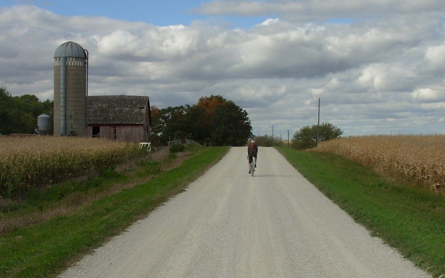
  \node[drop shadow={shadow xshift=0ex,shadow yshift=0ex},fill=white,draw] at (0,0) {\includegraphics[width=0.6\textwidth]{peeper.jpg}};
\end{tikzpicture}}
}

%%%%%%
\begin{frame}
\vspace{-0.3in}
\titlepage
\end{frame}

%%%%%%
\begin{frame}{What you'll learn about \hspace{0.2em}\includegraphics[width=0.07\textwidth]{Rlogo.jpg}}
\setbeamercovered{again covered={\opaqueness<1->{25}}}
\onslide<1->
\begin{itemize}
\itemsep12pt
\item What is R?
\item What's possible with R?
\begin{itemize}
\item CRAN and packages
\end{itemize}
\item R basics
\begin{itemize}
\item Installation
\item Command-line interface
\item Coding basics
\item Functions and objects
\item Data import and manipulation
\end{itemize}
\item Help!\\~\\
\end{itemize}
\pause
\Large
\centerline{\emph{Interactive!}}
\end{frame}


\section{Background}

%%%%%%
\begin{frame}{What is \includegraphics[width=0.07\textwidth]{Rlogo.jpg} \hspace{0.2em}? }
\setbeamercovered{again covered={\opaqueness<1->{25}}}
\onslide<1->
R is a language and environment for statistical computing and graphics
[\href{http://www.r-project.org/}{r-project.org}]\\~\\
\onslide<2->
R is a computer language that allows the user to program algorithms and use tools that
have been programmed by others [Zuur et al. 2009]\\~\\
\onslide<3->
Different from other statistics software because it is also a programming language...

\end{frame}

%%%%%%
\begin{frame}{What is \includegraphics[width=0.07\textwidth]{Rlogo.jpg} \hspace{0.2em}? }

\begin{center}
\begin{tikzpicture}
  \begin{scope}

    % The transparency:
    \begin{scope}[fill opacity=0.5]
      \fill[blue] (-2,0) circle (2.5);
      \fill[green] (2,0) circle (2.5);
    \end{scope}
    
    % letterings and missing pieces:
    \draw[align=center] (-2,0) circle (2.5) node[scale=1.2] {Programming};
    \draw[align=center] (2,0) circle (2.5) node[scale=1.2] {Statistics};
 		\draw (0,0) node[scale=2] {R};
 		
  \end{scope}
\end{tikzpicture}\\~\\
R is both... this creates a steep learning curve.
\end{center}
\end{frame}


%%%%%%
\begin{frame}[t]{What is \includegraphics[width=0.07\textwidth]{Rlogo.jpg} \hspace{0.2em}? }
\vspace{-0.1in}
\begin{columns}
\begin{column}{0.4\textwidth}
R is becoming the statistical software of choice\\~\\
Plot of Google scholar hits over time for different software packages
[\href{http://r4stats.com/articles/popularity/}{r4stats.com}]
\end{column}
\begin{column}{0.5\textwidth}
\begin{center}
\includegraphics[width=1.1\textwidth]{r_google.png}
\end{center}
\end{column}
\end{columns}
\end{frame}

%%%%%%
\begin{frame}[t]{What is \includegraphics[width=0.07\textwidth]{Rlogo.jpg} \hspace{0.2em}? }
\vspace{-0.1in}
\begin{columns}
\begin{column}{0.4\textwidth}
R is becoming the statistical software of choice\\~\\
Exponential growth in number of contributed packages
[\href{http://r4stats.com/articles/popularity/}{r4stats.com}]
\end{column}
\begin{column}{0.5\textwidth}
\begin{center}
\includegraphics[width=1.1\textwidth]{r_package.png}
\end{center}
\end{column}
\end{columns}
\end{frame}

%%%%%%
\begin{frame}{What's possible with \includegraphics[width=0.07\textwidth]{Rlogo.jpg} \hspace{0.2em}? }
R is incredibly flexible, if you want something done, someone else has written the code...\\~\\
\onslide<2->
R is open-source software, which mean it's free and is supported by a large network of contributors - the Comprehensive R Network [\href{http://cran.us.r-project.org/}{CRAN}]\\~\\
\onslide<3->
CRAN is a collection of sites which carry identical material, consisting of the R distribution(s), the contributed extensions, documentation for R, and binaries [\href{http://cran.us.r-project.org/faqs.html}{R FAQ}]\\~\\
\onslide<4->
Basically a repository of R utilities that others have written \onslide<5->- the \href{http://cran.r-project.org/web/views/}{CRAN task views} contain descriptions of contributed packages by category
\end{frame}

%%%%%%
\begin{frame}[t]{What's possible with \includegraphics[width=0.07\textwidth]{Rlogo.jpg} \hspace{0.2em}? }
\begin{center}
\includegraphics{cran_view1.png}
\end{center}
\end{frame}

%%%%%%
\begin{frame}[t]{What's possible with \includegraphics[width=0.07\textwidth]{Rlogo.jpg} \hspace{0.2em}? }
\begin{center}
\includegraphics{cran_view2.png}
\end{center}
\end{frame}

%%%%%%
\begin{frame}[t,fragile]{What's possible with \includegraphics[width=0.07\textwidth]{Rlogo.jpg} \hspace{0.2em}? }
R has a base package that is included in installation, others are downloaded as needed\\~\\
<<echo=true,eval=false>>=
install.packages('newpackage')
@
\vspace{0.2in}
The base package will be sufficient for most of your needs - includes arithmetic, input/output, basic programming support, graphics, etc.\\~\\
Contributed packages will meet your other needs - now exceed 4000
\end{frame}

%%%%%%
\begin{frame}[t,fragile]{What's possible with \includegraphics[width=0.07\textwidth]{Rlogo.jpg} \hspace{0.2em}? }
<<eval=false,echo=true>>=
demo(package = .packages(all.available = TRUE))
@
List of demonstrations with available packages - examples from ggplot2 package
\begin{columns}
\begin{column}{0.5\textwidth}
\begin{center}
\includegraphics[width=\textwidth]{ggplot1.png}
\end{center}
\end{column}
\begin{column}{0.5\textwidth}
\begin{center}
\includegraphics[width=\textwidth]{ggplot3.png}
\end{center}
\end{column}
\end{columns}
\end{frame}

%%%%%%
\begin{frame}[t,fragile]{What's possible with \includegraphics[width=0.07\textwidth]{Rlogo.jpg} \hspace{0.2em}? }
<<eval=false,echo=true>>=
demo(package = .packages(all.available = TRUE))
@
List of demonstrations with available packages - examples from ggplot2 package
\begin{columns}
\begin{column}{0.5\textwidth}
\begin{center}
\includegraphics[width=\textwidth]{ggplot2.png}
\end{center}
\end{column}
\begin{column}{0.5\textwidth}
\begin{center}
\includegraphics[width=\textwidth]{ggplot4.png}
\end{center}
\end{column}
\end{columns}
\end{frame}

\section{Basics}
%%%%%%
\begin{frame}[t]{\includegraphics[width=0.07\textwidth]{Rlogo.jpg} \hspace{0.01in} basics}
Installation - visit \href{http://cran.us.r-project.org/}{r-project.org} and follow directions
\centerline{\includegraphics{download.png}}
\end{frame}

%%%%%%
\begin{frame}[t]{\includegraphics[width=0.07\textwidth]{Rlogo.jpg} \hspace{0.01in} basics}
Or visit \href{http://pbil.univ-lyon1.fr/Rweb/}{Rweb} for an online version (not recommended)
\centerline{\includegraphics{rweb.png}}
\end{frame}

%%%%%%
\begin{frame}[t]{\includegraphics[width=0.07\textwidth]{Rlogo.jpg} \hspace{0.01in} basics}
A text editor is highly recommended, e.g. \href{http://www.rstudio.com/}{RStudio}\\~\\
\centerline{\includegraphics[width=0.65\textwidth]{Rstudio.png}}
\end{frame}

%%%%%%
\begin{frame}[t]{\includegraphics[width=0.07\textwidth]{Rlogo.jpg} \hspace{0.01in} basics}
How is R different from Excel? \onslide<2-> R is a command-line interface\\~\\
\centerline{\includegraphics[width=0.7\textwidth]{command_line.png}}
\onslide<3>
\centerline{\emph{What next??}}
\end{frame}

%%%%%%
\begin{frame}[fragile]{\includegraphics[width=0.07\textwidth]{Rlogo.jpg} \hspace{0.01in} basics}
Lines of code are executed by R at the prompt (\textit{\texttt{>}})\\~\\
\onslide<2>
Enter the code and press enter, the output is returned\\~\\
<<echo=T,results=tex>>=
print('hello world!')
2+2
(2+2)/4
rep("a",4)
@

\end{frame}

%%%%%%
\begin{frame}[fragile]{\includegraphics[width=0.07\textwidth]{Rlogo.jpg} \hspace{0.01in} basics}
A disadvantage of code is that everything entered must be 100 \% correct
\begin{Schunk}
\begin{Sinput}
> 2+2a
\end{Sinput}
\begin{Soutput}
Error: unexpected symbol in "2+2a"
\end{Soutput}
\begin{Sinput}
> a
\end{Sinput}
\begin{Soutput}
Error: object 'a' not found
\end{Soutput}
\end{Schunk}
\onslide<2>
\vspace{0.2in}
But this enables a complete documentation of your workflow... \\~\\
...your code is a living document of your analyses.
\end{frame}

%%%%%%
\begin{frame}[t,fragile]{\includegraphics[width=0.07\textwidth]{Rlogo.jpg} \hspace{0.01in} basics}
Assigning data to R objects is critical for analysis\\~\\
\onslide<2>
Assignment is possible using \textit{\texttt{<-}} or \textit{\texttt{=}}\\~\\
<<eval=true,echo=true>>=
a<-1
2+a
a=1
2+a
a=2+2
a/4
@
\end{frame}

%%%%%%
\begin{frame}[t,fragile]{\includegraphics[width=0.07\textwidth]{Rlogo.jpg} \hspace{0.01in} basics}
Assigning data to R objects is critical for analysis\\~\\
More complex assignments are possible\\~\\
<<eval=true,echo=true>>=
a<-c(1,2,3,4)
a
a<-seq(1,4)
a
a<-c("a","b","c")
a
@
\end{frame}

%%%%%%
\begin{frame}[fragile]{\includegraphics[width=0.07\textwidth]{Rlogo.jpg} \hspace{0.01in} basics}
Anatomy of a function - functions perform tasks for you, much like in Excel
\begin{center}
\Large
function(arguments)
\end{center}
\onslide<2>
<<eval=true,echo=true>>=
c(1,2) #concatenate function
mean(c(1,2)) #mean function
seq(1,4) #create a sequence of values
@
\end{frame}

%%%%%%
\begin{frame}[fragile,t]{\includegraphics[width=0.07\textwidth]{Rlogo.jpg} \hspace{0.01in} basics}
Understanding classes of R \href{http://cran.r-project.org/doc/manuals/r-release/R-lang.html#Vector-objects}{objects} is necessary for analysis \\~\\
An object is any variable of interest that you want to work with\\~\\
The class defines the type of information the object contains\\~\\
\onslide<2>
Most common are `numeric' or `character' classes \\~\\
<<echo=true,eval=true>>=
class(1)
class("1")
@
\vspace{0.2in}
\pause
`Factors' are also common, define categorical variables
\end{frame}

%%%%%%
\begin{frame}[fragile,t]{\includegraphics[width=0.07\textwidth]{Rlogo.jpg} \hspace{0.01in} basics}
Understanding classes of R \href{http://cran.r-project.org/doc/manuals/r-release/R-lang.html#Vector-objects}{objects} is necessary for analysis \\~\\
The classes of an object defines a protocol for evaluating or organizing variables\\~\\
For example, we cannot add add two objects with different classes:\\~\\
<<echo=true,eval=false>>=
'1' + 1
@
\begin{Schunk}
\begin{Soutput}
Error in "1" + 1 : non-numeric argument to binary operator
\end{Soutput}
\end{Schunk}
\end{frame}

%%%%%%
\begin{frame}[fragile]{\includegraphics[width=0.07\textwidth]{Rlogo.jpg} \hspace{0.01in} basics}
Objects (and their classes) can be stored in the computer's memory in different ways - aka the workspace for your R session\\~\\
Most common structures are `vectors' and `data.frames'\\~\\
\onslide<2->
Vectors are a collection of objects of the same class (e.g., a column in a table), whereas a data frame is analogous to a table with rows and columns (e.g., collection of vectors)
\onslide<3->
\begin{columns}[t]
\begin{column}{0.45\textwidth}
<<echo=true,eval=true>>=
a<-c(1,2)
a
b<-c("a","b")
b
@
\end{column}
\onslide<4->
\begin{column}{0.45\textwidth}
<<>>=
c<-data.frame(a,b)
c
@
\end{column}
\end{columns}
\end{frame}

%%%%%%
\begin{frame}[t,fragile]{\includegraphics[width=0.07\textwidth]{Rlogo.jpg} \hspace{0.01in} basics}
How are data imported into R?\\~\\
R needs to know where the data are located on your computer:\\~\\
<<echo=true,results=tex,eval=false>>=
setwd("C:/projects/my_data/")
@
\vspace{0.2in}
This establishes a `working directory' for data import/export\\~\\
\onslide<2>
R can import almost any type of data but `spreadsheet' or text-based files are most common \\~\\
\end{frame}

%%%%%%
\begin{frame}[t,fragile]{\includegraphics[width=0.07\textwidth]{Rlogo.jpg} \hspace{0.01in} basics}
How are data imported into R?\\~\\
R can import Excel data using the RODBC package, but this is not simple\\~\\
\onslide<2>
The easiest approach is to format data in Excel then export to a .csv or .txt file
\begin{columns}
\begin{column}{0.43\textwidth}
\begin{center}
\includegraphics{my_dat.png}
\end{center}
\end{column}
\begin{column}{0.66\textwidth}
\begin{center}
\includegraphics{save_as.png}
\end{center}
\end{column}
\end{columns}
\end{frame}

%%%%%%
\begin{frame}[t,fragile]{\includegraphics[width=0.07\textwidth]{Rlogo.jpg} \hspace{0.01in} basics}
How are data imported into R?\\~\\
Use the read.table or read.csv functions to import the data, must be in your working directory\\~\\
\onslide<2>
<<echo=true,eval=true>>=
dat<-read.csv("my_data.csv",header=T)
dat
@
\end{frame}

%%%%%%
\begin{frame}[t,fragile]{\includegraphics[width=0.07\textwidth]{Rlogo.jpg} \hspace{0.01in} basics}
How are data imported into R?\\~\\
Use the read.table or read.csv functions to import the data, must be in your working directory\\~\\
<<echo=true,eval=true>>=
dat<-read.table("my_data.csv",sep=',',header=T)
dat
@
\end{frame}

%%%%%%
\begin{frame}[t,fragile]{\includegraphics[width=0.07\textwidth]{Rlogo.jpg} \hspace{0.01in} basics}
Imported data can be viewed several ways, view the whole object or parts \\~\\
Rows or columns can be obtained by indexing with brackets separated by a comma: data[row,column]
\begin{columns}[t]
\onslide<2->
\begin{column}{0.45\textwidth}
<<echo=true>>=
dat
@
\end{column}
\onslide<3>
\begin{column}{0.45\textwidth}
<<>>=
dat[1,] #row 1
dat[,2] #column 2
dat[4,1] #row 4, column 1
@
\end{column}
\end{columns}
\end{frame}

%%%%%%
\begin{frame}[t,fragile]{\includegraphics[width=0.07\textwidth]{Rlogo.jpg} \hspace{0.01in} basics}
Imported data can be viewed several ways, view the whole object or parts \\~\\
Access using column names or the attach function
\begin{columns}[t]
\begin{column}{0.49\textwidth}
<<echo=true>>=
dat$Value
dat[,'Value']
@
\end{column}
\begin{column}{0.49\textwidth}
<<>>=
attach(dat)
Value
@
\end{column}
\end{columns}
\vspace{0.3in}
\onslide<2>
Vectors can be indexed similarly as data frames\\~\\
<<>>=
Value[2]
@
\end{frame}

%%%%%%
\begin{frame}[t,fragile]{\includegraphics[width=0.07\textwidth]{Rlogo.jpg} \hspace{0.01in} basics}
Where to go for help?\\~\\
\begin{itemize}
\addtolength{\itemsep}{0.08in}
\item A user-friendly \href{http://www.statmethods.net/}{intro to R} \pause
\item Several good introductory texts are available - Zuur et al. 2009. A Beginner's Guide to R. Springer. \pause
\item \href{http://cran.r-project.org/doc/contrib/Short-refcard.pdf}{R cheatsheet} \pause
\item Google is your friend \pause
\item Help files for each function using `?function' - may or may not be helpful \pause
\item An \href{http://cran.r-project.org/doc/manuals/R-intro.html}{intro to R} - very detailed
\item Ask us!
\end{itemize}
\end{frame}

% \begin{frame}[shrink]{References}%[t,allowframebreaks]{References}
% \scriptsize
% \setbeamertemplate{bibliography item}{}
% \bibliographystyle{C:/Projects/LaTeX/bibtex_bst/apalike_mine}
% \bibliography{C:/Projects/LaTeX/ref_diss}
% \end{frame}

\end{document}

\documentclass[xcolor=svgnames]{beamer}
\usetheme{Boadilla}
\usecolortheme[named=ForestGreen]{structure}
\usepackage{graphicx}
\usepackage[final]{animate}
%\usepackage[colorlinks=true,urlcolor=blue,citecolor=blue,linkcolor=blue]{hyperref}
\usepackage{breqn}
\usepackage{xcolor}
\usepackage{booktabs}
\usepackage{tikz}
\usetikzlibrary{shadows,arrows,positioning}
\usepackage[noae]{Sweave}
\definecolor{links}{HTML}{2A1B81}
\hypersetup{colorlinks,linkcolor=links,urlcolor=links}
\usepackage{pgfpages}
%\pgfpagesuselayout{4 on 1}[letterpaper, border shrink = 5mm, landscape]

\tikzstyle{block} = [rectangle, draw, text width=7em, text centered, rounded corners, minimum height=3em, minimum width=7em, top color = white, bottom color=green!30,  drop shadow]

\begin{document}
\SweaveOpts{concordance=TRUE}

\title[R for Data Analysis]{\includegraphics[width=0.07\textwidth]{Rlogo.jpg} \hspace{0.2em} for Data Analysis}
\author[M. Beck and S. Berg]{Marcus W. Beck \and Sergey Berg}

\institute[UofM]{Department of Fisheries, Wildlife, and Conservation Biology \\ University of Minnesota, Twin Cities}

\date{May 21, 2013}

\titlegraphic{
\centerline{
\begin{tikzpicture}
  \node[fill=white,draw] at (0,0) {\includegraphics[width=0.6\textwidth]{peeper.jpg}};
\end{tikzpicture}}
}

%%%%%%
\begin{frame}
\vspace{-0.3in}
\titlepage
\end{frame}

\section{Background}

%%%%%%
\begin{frame}{What you'll learn about \hspace{0.2em}\includegraphics[width=0.07\textwidth]{Rlogo.jpg}}
\setbeamercovered{again covered={\opaqueness<1->{25}}}
\onslide<1->
\begin{itemize}
\itemsep20pt
\item Data organization
\item Data exploration and visualization
\begin{itemize}
\item Common functions
\item Graphing tools
\end{itemize}
\item Data analysis and hypothesis testing
\begin{itemize}
\item Common functions
\item Evaluation of output 
\item Graphing tools \\~\\
\end{itemize}
\end{itemize}
\pause
\Large
\centerline{\emph{Interactive! Interrupt me!}}
\end{frame}

\section{Data organization}

%%%%%%
\begin{frame}[fragile]{Data organization}
We'll use the same dataset we used in Excel, replicating the analyses\\~\\
First we have to import the data into our R `workspace' \\~\\
\pause
The workspace is a group of R objects that are loaded for our current session \\~\\
Data are loaded into the workspace by importing (or making within R) and assigning them to a variable (object) with a name of our choosing\\~\\
We can see what's loaded in our workspace:\\~\\
\pause
<<echo=true>>=
a<-c(1,2)
ls()
@
\end{frame}

%%%%%%
\begin{frame}[fragile]{Data organization}
\onslide<+->{Import the data following this workflow:}\\~\\
\begin{center}
\begin{tikzpicture}[node distance=2.5cm, auto, >=stealth]
	\onslide<2->{
	\node[block] (a) {1. Open data in Excel and clean};}
	\onslide<3->{
	\node[block] (b)  [right of=a, node distance=4.2cm] {2. Save data in `.csv' format};
 	\draw[->] (a) -- (b);}
 	\onslide<4->{
 	\node[block] (c)  [right of=b, node distance=4.2cm]  {3. Import in R using 'read.csv'};
 	\draw[->] (b) -- (c);}
\end{tikzpicture}
\end{center}
\begin{columns}[t]
\onslide<2->{
\begin{column}{0.33\textwidth}
\begin{itemize}
\item Column names should be simple
\item Ensure all data will be easy to read
\end{itemize}
\end{column}}
\onslide<3->{
\begin{column}{0.33\textwidth}
\begin{itemize}
\item File, Save as .csv
\item Creates a comma separated file that looks like a spreadsheet
\item One spreadsheet at a time
\end{itemize}
\end{column}}
\onslide<4->{
\begin{column}{0.33\textwidth}
\begin{itemize}
\item header = T
\item See ?read.csv for list of function options
\item Remember to assign a name
\end{itemize}
\end{column}}
\end{columns}
\end{frame}

%%%%%%
\begin{frame}[fragile,shrink]{Data organization}
If the data are a text file... open the text file, how are the columns separated?
\begin{itemize}
\item comma
\item tabs
\item space
\item arbitrary character\\~\\
\end{itemize}
\pause
Use the read.table function and identify the column delimiter:
<<echo=true>>=
setwd('C:/Documents/monitoring_workshop')
ls() 
dat<-read.table('RWBB Survey.txt',sep='\t',header=T)
ls() 
@
\end{frame}

%%%%%%
\begin{frame}[fragile]{Data organization}
Now that the data are in our workspace, let's explore!\\~\\
\pause
Did the data import correctly (rarely a problem)?\\~\\
<<echo=true,eval=false>>=
head(dat) #or tail(dat)
@
\scriptsize
<<echo=false>>=
head(dat) #or tail(dat)
@
\end{frame}

\section{Data exploration}

%%%%%%
\begin{frame}[fragile]{Data exploration}
What object class is the data?
<<>>=
class(dat)
@
\pause
What are the dimensions of the data frame?
<<>>=
dim(dat)
nrow(dat)
ncol(dat)
@
The data contain \Sexpr{nrow(dat)} rows and \Sexpr{ncol(dat)} columns, is this correct?
\end{frame}

%%%%%%
\begin{frame}[fragile]{Data exploration}
Can we get a summary of the data frame?
\pause
<<>>=
summary(dat)
@
\end{frame}

%%%%%%
\begin{frame}[fragile]{Data exploration}
Individual summmaries of variables are also possible\\~\\
How do we obtain variables of interest?
\small
<<>>=
names(dat)
@
\pause
\normalsize
We can get a variable directly using \$ or via indexing with [,]
\small
<<>>=
dat$Temperature
dat[,'Temperature'] #same as dat[,7]
@
\end{frame}

%%%%%%
\begin{frame}[fragile]{Data exploration}
Just as we had summaries of the data frame, we can get summaries of individual variables
<<>>=
summary(dat$Temperature)
@
\pause
Or more simplistically...
<<>>=
mean(dat$Temperature)
range(dat$Temperature)
unique(dat$Temperature)
@
\end{frame}

%%%%%%
\begin{frame}[fragile]{Data exploration}
Note that the classes of our variables affect how R functions interpet them\\~\\
For example, the summary function returns different information...\\~\\
\small
<<>>=
class(dat$Temperature)
summary(dat$Temperature)
class(dat$SiteName)
summary(dat$SiteName)
@
\end{frame}

%%%%%%
\begin{frame}[fragile,t]{Data exploration}
What about site-specific evaluations?  What if we want to look at the temperature only at Kelly?\\~\\
<<>>=
Kelly<-subset(dat, dat$SiteName=='Kelly')
@
\vspace{0.2in}
We've created a new object in our workspace that is our original data frame with sites only from Kelly\\~\\
\pause
<<>>=
dim(Kelly)
Kelly$SiteName
@

\end{frame}

%%%%%%
\begin{frame}[fragile,t]{Data exploration}
What about site-specific evaluations?  What if we want to look at the temperature only at Kelly?\\~\\
<<>>=
Kelly<-subset(dat, dat$SiteName=='Kelly')
@
\vspace{0.2in}
Now we can evaluate the temperature, for example, only at Kelly\\~\\
<<>>=
mean(Kelly$Temperature) #this is the same as all sites
@
\end{frame}

%%%%%%
\begin{frame}[fragile]{Data exploration}
What abour our restoration project?  Aren't we comparing the abundances of breeding birds between restored and reference sites? \\~\\
Let's start with our reference sites...
<<>>=
ref<-dat$Reference
summary(ref) #or summary(dat$Reference)
@
\pause
Now the restored sites...
<<>>=
rest<-dat$Restoration
summary(rest)
@
\end{frame}

\section{Data visualization}

%%%%%%
\begin{frame}[fragile]{Data visualization}
Textual summaries of our data are nice, but we should also visualize:
\begin{itemize}
\item How are our data distributed?
\item Are there any outliers or extreme observations?
\item How do our variables compare (to a reference, to one another, over time, etc.)?\\~\\
\end{itemize}
\pause
R has many built in functions for data exploration and plotting
\begin{itemize}
\item hist - plots a histogram (binned densities of continuous values)
\item qqplot - comparison of a variable to a normal distribution
\item barplot - for bar plots...
\item plot - bivariate comparison of two variables
\item Much, much more...
\end{itemize}
\end{frame}

%%%%%%
\begin{frame}[fragile]{Data visualization}
Let's examine the distribution of abundances for the breeding birds at our reference site\\~\\
\begin{columns}
\begin{column}{0.6\textwidth}
<<hist_ref,fig=true,width=6,height=5,include=false>>=
hist(ref) #or hist(dat$Reference)
@
\begin{center}
\includegraphics[width=\textwidth,trim=0in 0in 0.3in 0.3in]{R_for_data_analysis-hist_ref.pdf}
\end{center}
\end{column}
\begin{column}{0.4\textwidth}
\pause
14 of our reference sites have abundances between 0--5 breeding birds
\end{column}
\end{columns}
\end{frame}

%%%%%%
\begin{frame}[fragile]{Data visualization}
How does it compare to our restoration site?\\~\\
\begin{columns}
\begin{column}{0.6\textwidth}
<<hist_rest,fig=true,width=6,height=5,include=false>>=
hist(rest) #or hist(dat$Restoration)
@
\begin{center}
\includegraphics[width=\textwidth,trim=0in 0in 0.3in 0.3in]{R_for_data_analysis-hist_rest.pdf}
\end{center}
\end{column}
\begin{column}{0.4\textwidth}
\pause
Six of our reference sites have abundances between 10--15 breeding birds
\end{column}
\end{columns}
\end{frame}

%%%%%%
\begin{frame}[fragile]{Data visualization}
Now that we've seen the distribution, how can we compare directly?\\~\\
<<box,fig=true,width=6,height=5,include=false>>=
boxplot(ref,rest)
@
\begin{columns}
\begin{column}{0.6\textwidth}
\begin{center}
\includegraphics[width=\textwidth,trim=0in 0in 0.3in 0.3in]{R_for_data_analysis-box.pdf}
\end{center}
\end{column}
\begin{column}{0.4\textwidth}
\pause
Let's make it look better...
\end{column}
\end{columns}
\end{frame}

%%%%%%
\begin{frame}[fragile]{Data visualization}
Now that we've seen the distribution, how can we compare directly?\\~\\
<<box2,fig=true,width=6,height=5,include=false>>=
boxplot(ref,rest,names=c('Reference','Restoration'),
	ylab='Bird abundance',col=c('lightblue','lightgreen'),
	main='Comparison of abundances between sites')
@
\begin{columns}
\begin{column}{0.6\textwidth}
\pause
\begin{center}
\includegraphics[width=\textwidth,trim=0in 0in 0.3in 0.3in]{R_for_data_analysis-box2.pdf}
\end{center}
\end{column}
\begin{column}{0.4\textwidth}
\pause
Dark line is median, box is 25$^{th}$ to 75$^{th}$ quartile (or IQR), whiskers are 1.5 $\times$ IQR\\~\\
Beyond can be considered outliers...
\end{column}
\end{columns}
\end{frame}

%%%%%%
\begin{frame}[fragile]{Data visualization}
What's going on with the outlier at our reference site?  How can we identify it? \\~\\
We can use the boxplot function for the dirty work...\\~\\
\pause
<<>>=
myplot<-boxplot(ref,rest)
myplot$out
@
\vspace{0.2in}
This gives us the actual value, now we need to find it in our data frame \\~\\
\pause
<<>>=
outlier<-myplot$out
out.row<-which(ref==outlier) 
out.row #this is the row number
@
\end{frame}

%%%%%%
\begin{frame}[fragile]{Data visualization}
<<eval=false>>=
dat[out.row,] #same as dat[8,]
@
\scriptsize
<<echo=false>>=
dat[out.row,] #same as dat[8,]
@
\vspace{0.2in}
\normalsize
Now we know that our outlier was from Kelly in 2007...\\~\\
What's odd about this record? \\~\\
\pause
Let's look at our records from Kelly...\\~\\
\end{frame}

%%%%%%
\begin{frame}[fragile]{Data visualization}
<<eval=false>>=
Kelly
@
\scriptsize
<<echo=false>>=
Kelly
@
\normalsize
\vspace{0.2in}
\pause
2007 was cold and rainy, could that have been the reason?\\~\\
Let's look at 2007 for all sites...
\end{frame}

%%%%%%
\begin{frame}[fragile]{Data visualization}
<<eval=false>>=
subset(dat,dat$Year=='2007')
@
\pause
\scriptsize
<<echo=false>>=
subset(dat,dat$Year=='2007')
@
\normalsize
\vspace{0.2in}
\pause
IGH and Carlton don't have high abundances at their reference sites during 2007 even though the weather was the same \\~\\
What else could have caused this outlier?\\~\\
\pause
<<eval=false>>=
summary(dat$ObserverNames)
@
\pause
\scriptsize
<<echo=false>>=
summary(dat$ObserverNames)
@
\end{frame}

%%%%%%
\begin{frame}[fragile]{Data visualization}
<<eval=false>>=
summary(dat$ObserverNames)
@
\scriptsize
<<echo=false>>=
summary(dat$ObserverNames)
@
\normalsize
\vspace{0.2in}
This is probably Jeremy and/or Lucy's fault, most likely switched the restoration and reference records \\~\\
\pause
What to change?
\pause
<<eval=false>>=
dat[out.row,'Restoration']<-18
dat[out.row,'Reference']<-2
@
Or...
<<eval=true>>=
dat<-dat[-out.row,] #do this one
@
Or...
fire Jeremy and Lucy.
\end{frame}

\section{Data analysis and hypothesis testing}

%%%%%%
\begin{frame}{Data analysis and hypothesis testing}
Now we need to evaluate the statistical certainty of our data, i.e., are our results due to random chance and how can we quantify this?\\~\\
\begin{columns}
\begin{column}{0.5\textwidth}
\begin{center}
\includegraphics[width=\textwidth,trim=0in 0in 0.3in 0.3in]{R_for_data_analysis-box2.pdf}
\end{center}
\end{column}
\begin{column}{0.5\textwidth}
\pause
We want to determine if the abundance of birds or variation among sites is actual or random\\~\\
\end{column}
\end{columns}
\pause
\centerline{What is an appropriate hypothesis?}
\end{frame}

<<hyp1,fig=T,include=false,eval=true,width=3.5,height=4.5,echo=false>>=
boxplot(dat$Reference,col='lightblue',main='Boxplot of abundance\nat reference sites',ylab='Bird abundance',ylim=c(-1,8))
abline(h=0,lty=2,lwd=2)
@

%%%%%%
\begin{frame}{Data analysis and hypothesis testing}
\centerline{What is an appropriate hypothesis? Let's start simple...}
\vspace{0.2in}
\pause
\begin{columns}
\begin{column}{0.5\textwidth}
\begin{block}{Null hypothesis}
The mean abundance of breeding birds at our reference site is zero.
\end{block}
\pause
\vspace{0.2in}
\begin{block}{Alternative hypothesis}
The mean abundance of breeding birds at our reference site is not zero.
\end{block}
\end{column}
\begin{column}{0.5\textwidth}
\pause
\centerline{\includegraphics[width=0.85\textwidth,trim=0in 0.8in 0in 0in]{R_for_data_analysis-hyp1.pdf}}
\end{column}
\end{columns}
\end{frame}

%%%%%%
\begin{frame}[t,fragile]{Data analysis and hypothesis testing}
The t.test function lets us test this hypothesis, very simple...\\~\\
<<eval=false>>=
t.test(dat$Reference)
@
\pause
\small
<<echo=false>>=
t.test(dat$Reference)
@
\normalsize
\vspace{0.2in}
\pause
What does this mean? \pause What are default arguments?\\~\\
\end{frame}

%%%%%%
\begin{frame}[t]{Data analysis and hypothesis testing}
Perhaps a one-tailed alternative hypothesis is better, we have prior assumptions about the data...\\~\\
\pause
\begin{columns}
\begin{column}{0.5\textwidth}
\begin{block}{Null hypothesis}
The mean abundance of breeding birds at our reference site is zero.
\end{block}
\pause
\vspace{0.2in}
\begin{block}{Alternative hypothesis}
The mean abundance of breeding birds at our reference site is greater than zero.
\end{block}
\end{column}
\begin{column}{0.5\textwidth}
\pause
\centerline{\includegraphics[width=0.85\textwidth,trim=0in 0.8in 0in 0in]{R_for_data_analysis-hyp1.pdf}}
\end{column}
\end{columns}
\end{frame}

%%%%%%
\begin{frame}[fragile]{Data analysis and hypothesis testing}
Slight modification of alternative argument for one-tailed test, default is two-tailed\\~\\
<<eval=false>>=
t.test(dat$Reference, alternative='greater')
@
\pause
\small
<<echo=false>>=
t.test(dat$Reference, alternative='greater')
@
\normalsize
\pause
What does this mean?
\end{frame}

<<hyp2,fig=T,include=false,eval=true,width=3.5,height=4.5,echo=false>>=
boxplot(dat$Reference,col='lightblue',main='Boxplot of abundance\nat reference sites',ylab='Bird abundance',ylim=c(-1,8))
abline(h=4,lty=2,lwd=2)
@

%%%%%%
\begin{frame}[t]{Data analysis and hypothesis testing}
Let's explore more flexibility of the t.test function by changing our basis of comparison for the alternative hypothesis\\~\\
\pause
\begin{columns}
\begin{column}{0.5\textwidth}
\begin{block}{Null hypothesis}
The mean abundance of breeding birds at our reference site is four.
\end{block}
\pause
\vspace{0.2in}
\begin{block}{Alternative hypothesis}
The mean abundance of breeding birds at our reference site is greater than four.
\end{block}
\end{column}
\begin{column}{0.5\textwidth}
\pause
\centerline{\includegraphics[width=0.85\textwidth,trim=0in 0.8in 0in 0in]{R_for_data_analysis-hyp2.pdf}}
\end{column}
\end{columns}
\end{frame}

%%%%%%
\begin{frame}[fragile,t]{Data analysis and hypothesis testing}
Test a different alternative hypothesis by changing the mu argument\\~\\
<<eval=false>>=
t.test(dat$Reference, mu=4, alternative='greater')
@
\pause
\small
<<echo=false>>=
t.test(dat$Reference, mu=4, alternative='greater')
@
\pause
\normalsize
What does this mean?
\end{frame}

%%%%%%
\begin{frame}{Data analysis and hypothesis testing}
Now the real question, let's compare our sites to one another...\\~\\
What are our hypotheses?\\~\\
\pause
\begin{columns}
\begin{column}{0.5\textwidth}
\begin{block}{Null hypothesis}
Differences in the mean abundance between restoration and reference sites is zero.
\end{block}
\pause
\vspace{0.2in}
\begin{block}{Alternative hypothesis}
Differences in the mean abundance between restoration and reference sites will be greater than zero.
\end{block}
\end{column}
\begin{column}{0.5\textwidth}
\pause
\centerline{\includegraphics[width=0.85\textwidth,trim=0in 1in 0.5in 0.5in]{R_for_data_analysis-box2.pdf}}
\end{column}
\end{columns}
\end{frame}

%%%%%%
\begin{frame}[fragile]{Data analysis and hypothesis testing}
Use the t.test function again as a two-sample test, order matters as do arguments\\~\\
<<eval=false>>=
t.test(dat$Restoration,dat$Reference,
	alternative='greater',var.equal=T)
@
\pause
\small
<<echo=false>>=
t.test(dat$Restoration,dat$Reference,
	alternative='greater',var.equal=T)
@
\normalsize
\pause
What does this mean?
\end{frame}

%%%%%%
\begin{frame}[fragile]{Data analysis and hypothesis testing}
Order of arguments matters...\\~\\
<<eval=false>>=
t.test(dat$Reference,dat$Restoration,
	alternative='greater',var.equal=T)
@
\pause
\small
<<echo=false>>=
t.test(dat$Reference,dat$Restoration,
	alternative='greater',var.equal=T)
@
\normalsize
\pause
What does this mean? \pause What happens if we change the alternative argument?
\end{frame}

%%%%%
\begin{frame}{Data analysis and hypothesis testing}
Our results suggest that the abundance of breeding birds at the restoration site is significantly greater than at the reference site
\pause
\vspace{0.5in}
\begin{columns}
\begin{column}{0.5\textwidth}
\centerline{\includegraphics[width=0.85\textwidth,trim=0in 1in 0.5in 0.5in]{R_for_data_analysis-box2.pdf}}
\end{column}
\begin{column}{0.5\textwidth}
Our p-value is 4.006e-06, what does this mean?\\~\\ 
\pause
There is a 0.0004006\% chance that our results were observed due to randomness (within the constraints of our test).
\end{column}
\end{columns}
\end{frame}

%%%%%%
\begin{frame}[t]{Data analysis and hypothesis testing}
Other common tests:\\~\\
\begin{itemize}
\itemsep20pt
\item $\chi^2$ test of independence - chisq.test
\item analysis of variance - anova or aov
\item correlations - cor.test or cor
\item regression - lm or glm 
\item Much, much more....
\end{itemize}
\end{frame}

%%%%%
\begin{frame}{Data analysis and hypothesis testing}
One last example... we've used common tests to compare our data to a standard or reference (e.g., mean is zero, differences in means is greater than zero)\\~\\
What about a more interesting analysis, such as comparison of data over time or relationships between variables?\\~\\
We'll close by illustrating use of linear regression with our data\\~\\
This is an evaluation of the mean response of a variable conditional on another, i.e., a predictor
\end{frame}

<<reg1,fig=true,include=false,eval=true,echo=false,width=4,height=4>>=
par(mar=c(4,4,0.5,0.5))
plot(Restoration~Year,data=dat)
@

%%%%%%
\begin{frame}[fragile]{Data analysis and hypothesis testing}
Perhaps we expect the abundance of breeding birds to increase at our restoration site over time, let's plot it:\\~\\
<<eval=false>>=
plot(Restoration~Year,data=dat)
@
\vspace{-0.13in}
\pause
\begin{columns}
\begin{column}{0.5\textwidth}
The first argument is entered as a `formula' specifying the variables\\~\\
The data argument specifies location of the variables in the workspace
\end{column}
\begin{column}{0.5\textwidth}
\begin{center}
\includegraphics[width=0.9\textwidth]{R_for_data_analysis-reg1.pdf}
\end{center}
\end{column}
\end{columns}
\end{frame}

<<reg2,fig=true,include=false,eval=true,echo=false,width=4,height=4>>=
par(mar=c(4,4,0.5,0.5))
plot(dat$Year,dat$Restoration)
@

%%%%%%
\begin{frame}[fragile]{Data analysis and hypothesis testing}
We can also call the variables directly in the plot function, x variable first, y second:\\~\\
<<eval=false>>=
plot(dat$Year,dat$Restoration)
@
\vspace{-0.13in}
\begin{columns}
\begin{column}{0.5\textwidth}
\onslide<2->
Note the change of the x and y labels, we can modify these using the xlab and ylab arguments in the plot function\\~\\
\onslide<3->
Notice the clear trend...
\end{column}
\begin{column}{0.5\textwidth}
\onslide<2->
\begin{center}
\includegraphics[width=0.9\textwidth]{R_for_data_analysis-reg2.pdf}
\end{center}
\end{column}
\end{columns}
\end{frame}

%%%%%%
\begin{frame}[fragile]{Data analysis and hypothesis testing}
How do we quantify this trend across time? Use the lm function for regression...\\~\\
<<eval=false>>=
lm(Restoration~Year,data=dat)
@
\pause
<<echo=false>>=
lm(Restoration~Year,data=dat)
@
\vspace{0.2in}
\pause
The abundance increases, on average, by \Sexpr{round(lm(Restoration~Year,data=dat)$coefficients[2],3)} birds per year.
\end{frame}

%%%%%%
\begin{frame}[fragile]{Data analysis and hypothesis testing}
We can get more information using the summary command 
\vspace{0.1in}
<<eval=false>>=
mod<-lm(Restoration~Year,data=dat)
summary(mod)
@
\pause
\scriptsize
<<echo=false>>=
mod<-lm(Restoration~Year,data=dat)
summary(mod)
@
\end{frame}

%%%%%%
\begin{frame}[fragile]{Data analysis and hypothesis testing}
What does this mean?
\vspace{0.1in}
\scriptsize
<<echo=false>>=
mod<-lm(Restoration~Year,data=dat)
summary(mod)
@
\end{frame}

<<reg3,fig=true,include=false,eval=true,echo=false,width=4,height=4>>=
par(mar=c(4,4,0.5,0.5))
plot(Restoration~Year, data=dat)
abline(reg=mod)
@

%%%%%%
\begin{frame}[fragile]{Data analysis and hypothesis testing}
How do we plot the model?\\~\\
<<eval=false>>=
plot(Restoration~Year, data=dat)
abline(reg=mod)
@
\vspace{-0.3in}
\begin{columns}
\begin{column}{0.5\textwidth}
We tell the abline function to plot our model, named `mod'
\end{column}
\begin{column}{0.5\textwidth}
\pause
\begin{center}
\includegraphics[width=0.9\textwidth]{R_for_data_analysis-reg3.pdf}
\end{center}
\end{column}
\end{columns}
\end{frame}

%%%%%
\begin{frame}[fragile]{Data analysis and hypothesis testing}
Can we use our model for prediction?\\~\\
What are the predicted data for our observation years?\\~\\
<<eval=false>>=
predict(mod)
@
\scriptsize
\pause
<<echo=false>>=
predict(mod)
@
\vspace{0.2in}
\normalsize
\pause
What about other years not in our dataset?
\end{frame}

%%%%%
\begin{frame}[fragile]{Data analysis and hypothesis testing}
Can we use our model for prediction?\\~\\
What about predicted abundance for 2011?\\~\\
<<eval=false>>=
predict(mod,newdata=data.frame(Year=2011))
@
\pause
<<echo=false>>=
predict(mod,newdata=data.frame(Year=2011))
@
\vspace{0.2in}
We can expect, on average, \Sexpr{round(predict(mod,newdata=data.frame(Year=2011)),2)} birds at our restoration sites in 2011 (within the constraints of our model)
\end{frame}

\section{Conclusion}

%%%%%
\begin{frame}{Conclusion}
What we've learned:\\~\\
\begin{itemize}
\itemsep20pt
\item Data organization - read.csv, read.table
\item Data exploration - head, dim, nrow, ncol, summary, [,], \$, names, subset, mean, range, unique
\item Data visualization - hist, boxplot, plot, abline
\item Data analysis and hypothesis testing - t.test, lm, predict\\~\\
\end{itemize}
\LARGE
\centerline{\emph{Questions?}}
\end{frame}

\end{document}

Integration take two – Shiny application

My last post discussed a technique for integrating functions in R using a Monte Carlo or randomization approach. The mc.int function (available here) estimated the area underneath a curve by multiplying the proportion of random points below the curve by the total area covered by points within the interval:

The estimated integration (bottom plot) is not far off from the actual (top plot). The estimate will converge on the actual as the point count reaches infinity. A useful feature of the function is the ability to visualize the integration of a model with no closed form solution for the anti-derivative, such as a loess smooth. I return to the idea of visualizing integrations for this blog using an alternative approach to estimate an integral. I’ve also incorporated this new function using a Shiny interface that allows the user to interactively explore the integration of different functions. I’m quite happy with how it turned out and I think the interface could be useful for anyone trying to learn integration.

The approach I use in this blog estimates an integral using a quadrature or column-based technique (an example). You’ll be familiar with this method if you’ve ever taken introductory calculus. The basic approach is to estimate the integral by summing the area of columns or rectangles that fill the approximate area under the curve. The accuracy of the estimate increases with decreasing column width such that the estimate approaches the actual value as column width approaches zero. An advantage of the approach is ease of calculation. The estimate is simply the sum of column areas determined as width times height. As in my last blog, this is a rudimentary approach that can only approximate the actual integral. R has several methods to more quantitatively approximate an integration, although options for visualization are limited.

The following illustrates use of a column-based approach such that column width decreases over the range of the interval:

The figure illustrates the integral of a standard normal curve from -1.96 to 1.96. We see that the area begins to approximate 0.95 with decreasing column width. All columns are bounded by the integral and the midpoint of each column is centered on an observed value from the function. The figures were obtained using the column.int function developed for this blog, which can be imported into your workspace as follows:

require(devtools)
source_gist(5568685)

In addition to the devtools package (to import from github), you’ll need to have the ggplot2, scales (which will install with ggplot2), and gridExtra packages installed. You’ll be prompted to install the packages if you don’t have them. Once the function is loaded in your workspace, you can run it as follows (using the default arguments):

column.int()

The function defaults to a standard normal curve integrated from -1.96 to 1.96 using twenty columns. The estimated area is projected as the plot title. The arguments for the function as are as follows:

int.fun	function to be integrated, entered as a character string or as class function, default ‘dnorm(x)’
num.poly	numeric vector indicating number of columns to use for integration, default 20
from.x	numeric vector indicating starting x value for integration, default -1.96
to.x	numeric vector indicating ending x value for integration, default 1.96
plot.cum	logical value indicating if a second plot is included that shows cumulative estimated integration with increasing number of columns up to num.poly, default FALSE

The plot.cum argument allows us to visualize the accuracy of our estimated integration. A second plot is included that shows the integration obtained from the integrate function (as a dashed line and plot title), as well as the integral estimate with increasing number of columns from one to num.poly using the column.int function. Obviously we would like to have enough columns to ensure our estimate is reasonably accurate.

column.int(plot.cum=T)

Our estimate converges rapidly to 0.95 with increasing number of columns. The estimated value will be very close to 0.95 with decreasing column width but be aware that computation time increases exponentially. An estimate with 20 columns takes less than a quarter second, whereas an estimate with 1000 columns takes 2.75 seconds. If we include a cumulative plot (plot.cum=T), the processing time is 0.47 seconds for 20 columns and three minutes 37 seconds for 1000 columns. Also be aware that the accuracy of the estimate will vary depending on the function. For the normal function, it’s easy to see how columns provide a reasonable approximation of the integral. This may not be the case for other functions:

column.int('sin(x^2)',n=5,from.x=-3,to.x=3,plot.cum=T)

Increasing the number of columns would be a good idea:

column.int('sin(x^2)',n=100,from.x=-3,to.x=3,plot.cum=T)

Now that you’ve got a feel for the function, I’ll introduce the Shiny interface. As an aside, this is my first attempt using Shiny and I am very impressed with its functionality. Much respect to the creators for making this application available. You can access the interface clicking the image below:

If you prefer, you can also load the interface locally one of two ways:

require(devtools)

shiny::runGist("https://gist.github.com/fawda123/5564846")

shiny::runGitHub('shiny_integrate', 'fawda123')

You can also access the code for the original function below. Anyhow, I hope this is useful to some of you. I would be happy to entertain suggestions for improving the functionality of this tool.

-Marcus

column.int<-function(int.fun='dnorm(x)',num.poly=20,from.x=-1.96,to.x=1.96,plot.cum=F){
	
	if (!require(ggplot2) | !require(scales) | !require(gridExtra)) {
	  stop("This app requires the ggplot2, scales, and gridExtra packages. To install, run 'install.packages(\"name\")'.\n")
	}
 
	if(from.x>to.x) stop('Starting x must be less than ending x')
	
	if(is.character(int.fun)) int.fun<-eval(parse(text=paste('function(x)',int.fun)))
	
	int.base<-0	
	poly.x<-seq(from.x,to.x,length=num.poly+1)
	
	polys<-sapply(
	  1:(length(poly.x)-1),
		function(i){
			
			x.strt<-poly.x[i]
			x.stop<-poly.x[i+1]
			
			cord.x<-rep(c(x.strt,x.stop),each=2) 
			cord.y<-c(int.base,rep(int.fun(mean(c(x.strt,x.stop))),2),int.base) 
			data.frame(cord.x,cord.y)
	
			},
		simplify=F
		)
	
	area<-sum(unlist(lapply(
		polys,
		function(x) diff(unique(x[,1]))*diff(unique(x[,2]))
		)))
	txt.val<-paste('Area from',from.x,'to',to.x,'=',round(area,4),collapse=' ')
	
	y.col<-rep(unlist(lapply(polys,function(x) max(abs(x[,2])))),each=4)
	plot.polys<-data.frame(do.call('rbind',polys),y.col)
	
	p1<-ggplot(data.frame(x=c(from.x,to.x)), aes(x)) + stat_function(fun=int.fun)
	if(num.poly==1){ 
		p1<-p1 + geom_polygon(data=plot.polys,mapping=aes(x=cord.x,y=cord.y),
			alpha=0.7,color=alpha('black',0.6))
		}
	else{
		p1<-p1 + geom_polygon(data=plot.polys,mapping=aes(x=cord.x,y=cord.y,fill=y.col,
			group=y.col),alpha=0.6,color=alpha('black',0.6))
		}
	p1<-p1 + ggtitle(txt.val) + theme(legend.position="none") 
	
	if(!plot.cum) print(p1)
	
	else{
		
		area.cum<-unlist(sapply(1:num.poly,
			function(val){
				poly.x<-seq(from.x,to.x,length=val+1)
				
				polys<-sapply(
				  1:(length(poly.x)-1),
					function(i){
						
						x.strt<-poly.x[i]
						x.stop<-poly.x[i+1]
						
						cord.x<-rep(c(x.strt,x.stop),each=2) 
						cord.y<-c(int.base,rep(int.fun(mean(c(x.strt,x.stop))),2),int.base) 
						data.frame(cord.x,cord.y)
				
						},
					simplify=F
					)
				
				sum(unlist(lapply(
					polys,
					function(x) diff(unique(x[,1]))*diff(unique(x[,2]))
					)))
				
				}
			))
		
		dat.cum<-data.frame(Columns=1:num.poly,Area=area.cum)
		actual<-integrate(int.fun,from.x,to.x)
		
		p2<-ggplot(dat.cum, aes(x=Columns,y=Area)) + geom_point()
		p2<-p2 + geom_hline(yintercept=actual$value,lty=2) 
		p2<-p2 + ggtitle(paste('Actual integration',round(actual$value,4),'with absolute error',prettyNum(actual$abs.error)))
		
		grid.arrange(p1,p2)
		
		}
	
	}

Poor man’s integration – a simulated visualization approach

Every once in a while I encounter a problem that requires the use of calculus. This can be quite bothersome since my brain has refused over the years to retain any useful information related to calculus. Most of my formal training in the dark arts was completed in high school and has not been covered extensively in my post-graduate education. Fortunately, the times when I am required to use calculus are usually limited to the basics, e.g., integration and derivation. If you’re a regular reader of my blog, you’ll know that I often try to make life simpler through the use of R. The focus of this blog is the presentation of a function that can integrate an arbitrarily-defined curve using a less than quantitative approach, or what I like to call, poor man’s integration. If you are up to speed on the basics of calculus, you may recognize this approach as Monte Carlo integration. I have to credit Dr. James Forester (FWCB dept., UMN) for introducing me to this idea.

If you’re like me, you’ll need a bit of a refresher on the basics of integration. Simply put, the area underneath a curve, bounded by some x-values, can be obtained through integration. Most introductory calculus texts will illustrate this concept using a uniform distribution, such as:

If we want to get the area of the curve between, for example 0.5 and 1.5, we find the area of the blue box:

Going back to basic geometry, we know that this is the width (1.5-0.5) multiplied by the height (0.5-0), or 0.5. In calculus terms, this means we’ve integrated the uniform function with the definite integral from 0.5 to 1.5. Integration becomes more complicated with increasingly complex functions and we can’t use simple geometric equations to obtain an answer. For example, let’s define our function as:

Now we want to integrate the function from -1 to 1 as follows:

Using calculus to find the area:

The integrated portion is the area of the curve from negative infinity to 1 minus the area from negative infinity to -1, where the area is determined based on the integrated form of the function, or the antiderivative. The integrate function in R can perform these calculations for you, so long as you define your function properly.

int.fun<-function(x) 1+x^2
integrate(int.fun,-1,1)

The integrate function will return the same value as above, with an indication of error for the estimate. The nice aspect about the integrate function is that it can return integral estimates if the antiderivative has no closed form solution. This is accomplished (from the help file) using ‘globally adaptive interval subdivision in connection with extrapolation by Wynn’s Epsilon algorithm, with the basic step being Gauss–Kronrod quadrature’. I’d rather take a cold shower than figure out what this means. However, I assume the integration involves summing the area of increasingly small polygons across the interval, something like this. The approach I describe here is similar except random points are placed in the interval, rather than columns. The number of points under the curve relative to total number of points is multiplied by the total area that the points cover. The integral estimation approximates the actual as the number of points approaches infinity. After creating this function, I realized that the integrate function can accomplish the same task. However, I’ve incorporated some plotting options for my function to illustrate how the integral is estimated.

Let’s start by creating an arbitrary model for integration. We’ll create random points and then approximate a line of best fit using the loess smoother.

set.seed(3)

x<-seq(1,10)
y<-runif(10,0,20)
dat<-data.frame(x,y)

model<-loess(y~x, data=dat)

The approximated loess model through our random points looks like this:

The antiderivative of the approximated model does not exist in a useful form since the loess function uses local fitting. We can use the integrate function to calculate the area under the curve. The integrate function requires as input a function that takes a numeric first argument and returns a numeric vector of the same length, so we have convert our model accordingly. We’ll approximate the definite integral from 4 to 8.

mod.fun<-function(x) predict(model,newdata=x)
integrate(mod.fun,4,8)

The function tells us that the area under the curve from 4 to 8 is 33.1073 with absolute error < 3.7e-13. Now we can compare this estimate to one obtained using my function. We'll import the mc.int function from Github.

require(devtools)
source_gist(5483807)

This function differs from integrate in a few key ways. The input is an R object model that has a predict (e.g., predict.lm) method, rather than an R function that returns a numeric vector the same length as the input. This is helpful because it eliminates the need to create your own prediction function for your model. Additionally, a plot is produced that shows the simulation data that were used to estimate the integral. Finally, the integration method uses randomly placed points rather than a polygon-based approach. I don’t know enough about integration to speak about the strength and weaknesses of either approach, but the point-based method is more straight-forward (in my opinion).

Let’s integrate our model from 4 to 8 using the mc.int function imported from Github.

mc.int(model,int=c(4,8),round.val=6)

The estimate returned by the function is 32.999005, which is very close to the estimate returned from integrate. The default behavior of mc.int is to return a plot showing the random points that were used to obtain the estimate:

All of the points in green were below the curve. The area where the points were randomly located (x = 4 to x = 8 and y=0 to y=14) was multiplied by the number of green points divided by the total number of points. The function has the following arguments:

mod.in	fitted R model object, must have predict method
int	two-element numeric vector indicating interval for integration, integrates function across its range if none provided
n	numeric vector indicating number of random points to use, default 10000
int.base	numeric vector indicating minimum y location for integration, default 0
plot	logical value indicating if results should be plotted, default TRUE
plot.pts	logical value indicating if random points are plotted, default TRUE
plot.poly	logical value indicating if a polygon representing the integration region should be plotted, default TRUE
cols	three-element list indicating colors for points above curve, points below curve, and polygon, default ‘black’,’green’, and ‘blue’
round.val	numeric vector indicating number of digits for rounding integration estimate, default 2
val	logical value indicating if only the estimate is returned with no rounding, default TRUE

Two characteristics of the function are worth noting. First, the integration estimate varies with the total number of points:

Second, the integration estimate changes if we run the function again with the same total number of points since the point locations are chosen randomly:

These two issues represent one drawback of the mc.int function because a measure of certainty is not provided with the integration estimate, unlike the integrate function. However, an evaluation of certainty for an integral with no closed form solution is difficult to obtain because the actual value is not known. Accordingly, we can test the accuracy and precision of the mc.int function to approximate an integral with a known value. For example, the integral of the standard normal distribution from -1.96 to 1.96 is 0.95.

The mc.int function will only be useful if it produces estimates for this integral that are close to 0.95. These estimates should also exhibit minimal variation with repeated random estimates. To evaluate the function, we’ll test an increasing number of random points used to approximate the integral, in addition to repeated number of random estimates for each number of random points. This allows an evaluation of accuracy and precision. The following code evaluated number of random points from 10 to 1000 at intervals of 10, with 500 random samples for each interval. The code uses another function, mc.int.ex, imported from Github that is specific to the standard normal distribution.

#import mc.int.ex function for integration of standard normal
source_gist(5484425)

#get accuracy estimates from mc.int.ex
rand<-500
check.acc<-seq(10,1000,by=10)
mc.dat<-vector('list',length(check.acc))
names(mc.dat)<-check.acc
for(val in check.acc){
	out.int<-numeric(rand)
	for(i in 1:rand){
		cat('mc',val,'rand',i,'\n')
		out.int[i]<-mc.int.ex(n=val,val=T)
		flush.console()
		}
	mc.dat[[as.character(val)]]<-out.int
	}

The median integral estimate, as well as the 2.5th and 97.5th quantile values were obtained for the 500 random samples at each interval (i.e., a non-parametric bootstrap approach). Plotting the estimates as a function of number of random points shows that the integral estimate approaches 0.95 and the precision of the estimate increases with increasing number of points. In fact, an estimate of the integral with 10000 random points and 500 random samples is 0.950027 (0.9333885, 0.9648904).

The function is not perfect but it does provide a reasonable integration estimate if the sample size is sufficiently high. I don’t recommend using this function in place integrate, but it may be useful for visualizing an integration. Feel free to use/modify as you see fit. Cheers!