
In my last post I said I wasn’t going to write anymore about neural networks (i.e., multilayer feedforward perceptron, supervised ANN, etc.). That was a lie. I’ve received several requests to update the neural network plotting function described in the original post. As previously explained, R does not provide a lot of options for visualizing neural networks. The only option I know of is a plotting method for objects from the neuralnet package. This may be my opinion, but I think this plot leaves much to be desired (see below). Also, no plotting methods exist for neural networks created in other packages, i.e., nnet and RSNNS. These packages are the only ones listed on the CRAN task view, so I’ve updated my original plotting function to work with all three. Additionally, I’ve added a new option for plotting a raw weight vector to allow use with neural networks created elsewhere. This blog describes these changes, as well as some new arguments added to the original function.

As usual, I’ll simulate some data to use for creating the neural networks. The dataset contains eight input variables and two output variables. The final dataset is a data frame with all variables, as well as separate data frames for the input and output variables. I’ve retained separate datasets based on the syntax for each package.
library(clusterGeneration)

seed.val<-2
set.seed(seed.val)

num.vars<-8
num.obs<-1000

#input variables
cov.mat<-genPositiveDefMat(num.vars,covMethod=c("unifcorrmat"))$Sigma
rand.vars<-mvrnorm(num.obs,rep(0,num.vars),Sigma=cov.mat)

#output variables
parms<-runif(num.vars,-10,10)
y1<-rand.vars %*% matrix(parms) + rnorm(num.obs,sd=20)
parms2<-runif(num.vars,-10,10)
y2<-rand.vars %*% matrix(parms2) + rnorm(num.obs,sd=20)

#final datasets
rand.vars<-data.frame(rand.vars)
resp<-data.frame(y1,y2)
names(resp)<-c('Y1','Y2')
dat.in<-data.frame(resp,rand.vars)
The various neural network packages are used to create separate models for plotting.
#nnet function from nnet package
library(nnet)
set.seed(seed.val)
mod1<-nnet(rand.vars,resp,data=dat.in,size=10,linout=T)

#neuralnet function from neuralnet package, notice use of only one response
library(neuralnet)
form.in<-as.formula('Y1~X1+X2+X3+X4+X5+X6+X7+X8')
set.seed(seed.val)
mod2<-neuralnet(form.in,data=dat.in,hidden=10)

#mlp function from RSNNS package
library(RSNNS)
set.seed(seed.val)
mod3<-mlp(rand.vars, resp, size=10,linOut=T)
I’ve noticed some differences between the functions that could lead to some confusion. For simplicity, the above code represents my interpretation of the most direct way to create a neural network in each package. Be very aware that direct comparison of results is not advised given that the default arguments differ between the packages. A few key differences are as follows, although many others should be noted. First, the functions differ in the methods for passing the primary input variables. The nnet function can take separate (or combined) x and y inputs as data frames or as a formula, the neuralnet function can only use a formula as input, and the mlp function can only take a data frame as combined or separate variables as input. As far as I know, the neuralnet function is not capable of modelling multiple response variables, unless the response is a categorical variable that uses one node for each outcome. Additionally, the default output for the neuralnet function is linear, whereas the opposite is true for the other two functions.
Specifics aside, here’s how to use the updated plot function. Note that the same syntax is used to plot each model.
#import the function from Github
library(devtools)
source_url('https://gist.githubusercontent.com/fawda123/7471137/raw/466c1474d0a505ff044412703516c34f1a4684a5/nnet_plot_update.r')

#plot each model
plot.nnet(mod1)
plot.nnet(mod2)
plot.nnet(mod3)

nnet object (mod1).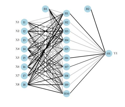
neuralnet object (mod2).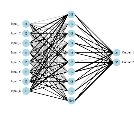
mlp object (mod3).
The neural networks for each model are shown above. Note that only one response variable is shown for the second plot. Also, neural networks created using mlp do not show bias layers, causing a warning to be returned. The documentation about bias layers for this function is lacking, although I have noticed that the model object returned by mlp does include information about ‘unitBias’ (see the output from mod3$snnsObject$getUnitDefinitions()). I wasn’t sure what this was so I excluded it from the plot. Bias layers aren’t all that informative anyway, since they are analogous to intercept terms in a regression model. Finally, the default variable labels differ for the mlp plot from the other two. I could not find any reference to the original variable names in the mlp object, so generic names returned by the function are used.
I have also added five new arguments to the function. These include options to remove bias layers, remove variable labels, supply your own variable labels, and include the network architecture if using weights directly as input. The new arguments are shown in bold.
mod.in |
neural network object or numeric vector of weights, if model object must be from nnet, mlp, or neuralnet functions |
nid |
logical value indicating if neural interpretation diagram is plotted, default T |
all.out |
character string indicating names of response variables for which connections are plotted, default all |
all.in |
character string indicating names of input variables for which connections are plotted, default all |
bias |
logical value indicating if bias nodes and connections are plotted, not applicable for networks from mlp function, default T |
wts.only |
logical value indicating if connections weights are returned rather than a plot, default F |
rel.rsc |
numeric value indicating maximum width of connection lines, default 5 |
circle.cex |
numeric value indicating size of nodes, passed to cex argument, default 5 |
node.labs |
logical value indicating if labels are plotted directly on nodes, default T |
var.labs |
logical value indicating if variable names are plotted next to nodes, default T |
x.lab |
character string indicating names for input variables, default from model object |
y.lab |
character string indicating names for output variables, default from model object |
line.stag |
numeric value that specifies distance of connection weights from nodes |
struct |
numeric value of length three indicating network architecture(no. nodes for input, hidden, output), required only if mod.in is a numeric vector |
cex.val |
numeric value indicating size of text labels, default 1 |
alpha.val |
numeric value (0-1) indicating transparency of connections, default 1 |
circle.col |
character string indicating color of nodes, default ‘lightblue’, or two element list with first element indicating color of input nodes and second indicating color of remaining nodes |
pos.col |
character string indicating color of positive connection weights, default ‘black’ |
neg.col |
character string indicating color of negative connection weights, default ‘grey’ |
max.sp |
logical value indicating if space between nodes in each layer is maximized, default F |
... |
additional arguments passed to generic plot function |
The plotting function can also now be used with an arbitrary weight vector, rather than a specific model object. The struct argument must also be included if this option is used. I thought the easiest way to use the plotting function with your own weights was to have the input weights as a numeric vector, including bias layers. I’ve shown how this can be done using the weights directly from mod1 for simplicity.
wts.in<-mod1$wts
struct<-mod1$n
plot.nnet(wts.in,struct=struct)
Note that wts.in is a numeric vector with length equal to the expected given the architecture (i.e., for 8 10 2 network, 100 connection weights plus 12 bias weights). The plot should look the same as the plot for the neural network from nnet.
The weights in the input vector need to be in a specific order for correct plotting. I realize this is not clear by looking directly at wt.in but this was the simplest approach I could think of. The weight vector shows the weights for each hidden node in sequence, starting with the bias input for each node, then the weights for each output node in sequence, starting with the bias input for each output node. Note that the bias layer has to be included even if the network was not created with biases. If this is the case, simply input a random number where the bias values should go and use the argument bias=F. I’ll show the correct order of the weights using an example with plot.nn from the neuralnet package since the weights are included directly on the plot.
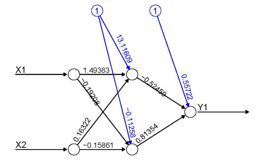
If we pretend that the above figure wasn’t created in R, we would input the mod.in argument for the updated plotting function as follows. Also note that struct must be included if using this approach.
mod.in<-c(13.12,1.49,0.16,-0.11,-0.19,-0.16,0.56,-0.52,0.81)
struct<-c(2,2,1) #two inputs, two hidden, one output
plot.nnet(mod.in,struct=struct)
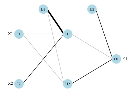
plot.nnet function by direct input of model weights.
Note the comparability with the figure created using the neuralnet package. That is, larger weights have thicker lines and color indicates sign (+ black, – grey).
One of these days I’ll actually put these functions in a package. In the mean time, please let me know if any bugs are encountered.
Cheers,
Marcus
Update:
I’ve changed the function to work with neural networks created using the train function from the caret package. The link above is updated but you can also grab it here.
mod4<-train(Y1~.,method='nnet',data=dat.in,linout=T)
plot.nnet(mod4,nid=T)
Also, factor levels are now correctly plotted if using the nnet function.
fact<-factor(sample(c('a','b','c'),size=num.obs,replace=T))
form.in<-formula('cbind(Y2,Y1)~X1+X2+X3+fact')
mod5<-nnet(form.in,data=cbind(dat.in,fact),size=10,linout=T)
plot.nnet(mod5,nid=T)
Update 2:
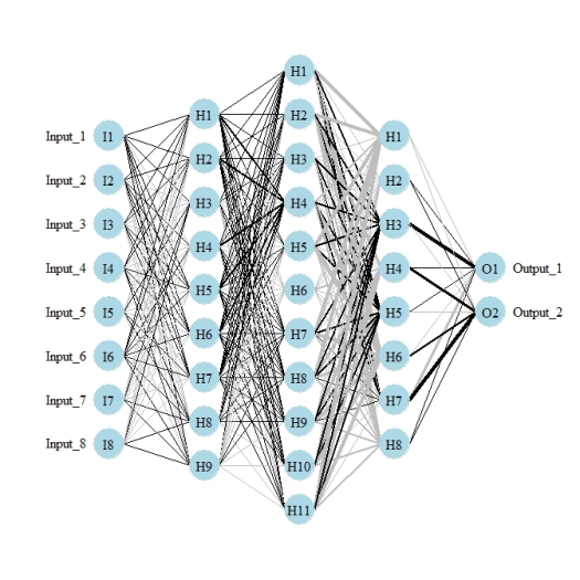
More updates… I’ve now modified the function to plot multiple hidden layers for networks created using the mlp function in the RSNNS package and neuralnet in the neuralnet package. As far as I know, these are the only neural network functions in R that can create multiple hidden layers. All others use a single hidden layer. I have not tested the plotting function using manual input for the weight vectors with multiple hidden layers. My guess is it won’t work but I can’t be bothered to change the function unless it’s specifically requested. The updated function can be grabbed here (all above links to the function have also been changed).
library(RSNNS)

#neural net with three hidden layers, 9, 11, and 8 nodes in each
mod<-mlp(rand.vars, resp, size=c(9,11,8),linOut=T)
par(mar=numeric(4),family='serif')
plot.nnet(mod)
plot.nnet function with multiple hidden layers from a network created with mlp.Here’s an example using the neuralnet function with binary predictors and categorical outputs (credit to Tao Ma for the model code).
library(neuralnet)

#response
AND<-c(rep(0,7),1)
OR<-c(0,rep(1,7))

#response with predictors
binary.data<-data.frame(expand.grid(c(0,1),c(0,1),c(0,1)),AND,OR)

#model
net<-neuralnet(AND+OR~Var1+Var2+Var3, binary.data,hidden=c(6,12,8),rep=10,err.fct="ce",linear.output=FALSE)

#plot ouput
par(mar=numeric(4),family='serif')
plot.nnet(net)
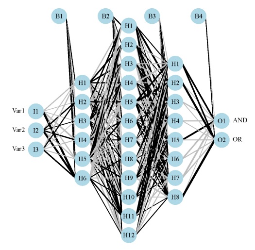
plot.nnet function with multiple hidden layers from a network created with neuralnet.Update 3:
The color vector argument (circle.col) for the nodes was changed to allow a separate color vector for the input layer. The following example shows how this can be done using relative importance of the input variables to color-code the first layer.
#example showing use of separate colors for input layer
#color based on relative importance using 'gar.fun'

##
#create input data
seed.val<-3
set.seed(seed.val)

num.vars<-8
num.obs<-1000

#input variables
library(clusterGeneration)
cov.mat<-genPositiveDefMat(num.vars,covMethod=c("unifcorrmat"))$Sigma
rand.vars<-mvrnorm(num.obs,rep(0,num.vars),Sigma=cov.mat)

#output variables
parms<-runif(num.vars,-10,10)
y1<-rand.vars %*% matrix(parms) + rnorm(num.obs,sd=20)

#final datasets
rand.vars<-data.frame(rand.vars)
resp<-data.frame(y1)
names(resp)<-'Y1'
dat.in<-data.frame(resp,rand.vars)

##
#create model
library(nnet)
mod1<-nnet(rand.vars,resp,data=dat.in,size=10,linout=T)

##
#relative importance function
library(devtools)
source_url('https://gist.github.com/fawda123/6206737/raw/2e1bc9cbc48d1a56d2a79dd1d33f414213f5f1b1/gar_fun.r')

#relative importance of input variables for Y1
rel.imp<-gar.fun('Y1',mod1,bar.plot=F)$rel.imp

#color vector based on relative importance of input values
cols<-colorRampPalette(c('green','red'))(num.vars)[rank(rel.imp)]

##
#plotting function
source_url('https://gist.githubusercontent.com/fawda123/7471137/raw/466c1474d0a505ff044412703516c34f1a4684a5/nnet_plot_update.r')

#plot model with new color vector
#separate colors for input vectors using a list for 'circle.col'
plot(mod1,circle.col=list(cols,'lightblue'))
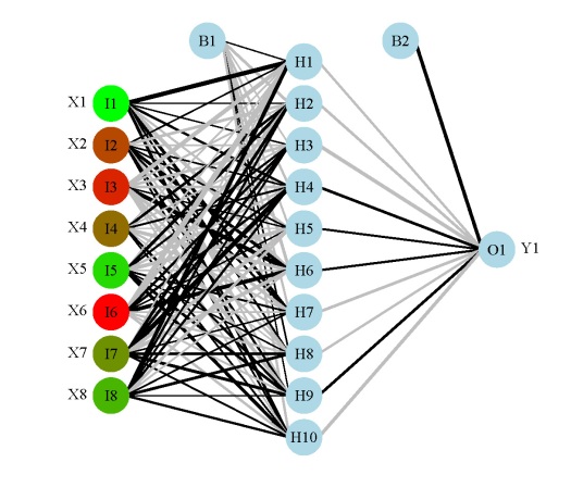
plot.nnet function with input nodes color-coded in relation to relative importance.