I’ve recently posted two blogs about gathering data from web pages using functions in R. Both examples showed how we can create our own custom functions to gather data about Minnesota lakes from the Lakefinder website. The first post was an example showing the use of R to create our own custom functions to get specific lake information and the second was a more detailed example showing how we can get data on fish populations in each lake. Each of the examples used functions in the XML package to parse the raw XML/HTML from the web page for each lake. I promised to show some results using information that was gathered with the catch function described in the second post. The purpose of this blog is to present some of this information and to further illustrate the utility of data mining using public data and functions in R.
I’ll begin by describing the functionality of a revised catch function and the data that can be obtained. I’ve revised the original function to return more detailed information and decrease processing time, so this explanation is not a repeat of my previous blog. First, we import the function from Github with some help from the RCurl package.
#import function from Github
require(RCurl)

root.url<-'https://gist.github.com/fawda123'
raw.fun<-paste(
  root.url,
  '4978092/raw/336671b8c3d44f744c3c8c87dd18e6d871a3b370/catch_fun_v2.r',
  sep='/'
  )

script<-getURL(raw.fun, ssl.verifypeer = FALSE)
eval(parse(text = script))
rm('script','raw.fun')

#function name 'catch.fun.v2'
The revised function is much simpler than the previous and requires only three arguments.
formals(catch.fun.v2)
#dows

#$trace
#T

#$rich.out
#F
The ‘dows’ argument is a character vector of the 8-digit lake identifier numbers used by MNDNR, ‘trace’ is a logical specifying if progress is returned as the function runs, and ‘rich.out’ is a logical specifying if a character vector of all fish species is returned as a single element list. The ‘dows’ argument can process multiple lakes so long as you have the numbers. The default value for the last argument will return a list of two data frames with complete survey information for each lake.
I revised the original function after realizing that I’ve made the task of parsing XML for individual species much too difficult. The original function searches species names and gear type to find the appropriate catch data. A simpler approach is to find the entire survey table by parsing with <table></table> tags. The original function parsed the XML using <tr></tr> tags for table rows and then identified the appropriate species and gear type within the rows. The latter approach required multiple selection criteria and was incredibly inefficient. The new function returns entire tables, which can be further modified within R as needed. Here’s an example for Loon lake in Aitkin county.
catch.fun.v2('01002400')

#01002400; 1 of 1
#Time difference of 1.844106 secs
#$`01002400`
#$`01002400`$abundance
#Species        Net Caught Ave_wt
#1  White Sucker  Trap net     0.1   ND
#2 Rainbow Trout  Trap net   trace   ND
#3   Brook Trout  Trap net     4.6   ND

#$`01002400`$length
#Species   0-5   6-8  9-11 12-14 15-19
#1   Brook Trout     0    28    36    22     3
#2 Rainbow Trout     0     0     0     1     0
#20-24 25-29   30+  Total
#1     0     0     0     89
#2     0     0     0      1
This is the same information that is on the lakefinder website. A two-element list is returned for each lake, each containing a data frame. The first element is a data frame of species catch (fish per net) and average weight (lbs per fish) using trap nets and gill nets (this example only contained trap nets). The second element is a length distribution table showing the number of fish caught within binned length categories (inches). A character string specifying ‘No survey’ will be returned if the lake isn’t found on the website or if no fish surveys are available. A character string indicating ‘No length table’ will be returned in the second list element if only the abundance table is available.
A list of the species present is returned if ‘rich.out’ is true.
catch.fun.v2('01002400',rich.out=T)

#01002400; 1 of 1
#Time difference of 0.419024 secs
#$`01002400`
#[1] "Brook Trout"   "Rainbow Trout"
#[3] "White Sucker"
Clearly the utility of this function is the ability to gather lake data for multiple lakes without visiting each individual page on Lakefinder. I’ve used the function to get lake data for every lake on the website. The dow numbers were obtained from a publicly available shapefile of lakes in Minnesota. This included 17,085 lakes, which were evaluated by the function in less than an hour. Of these lakes, 3,934 had fish survey information. One drawback of the function is that I haven’t included the date of the survey in the output (updated, see link at bottom of blog). The data that are returned span several years, and in some cases, the most recent lake survey could have been over 40 years ago.
Below is a presentation of some of the more interesting information obtained from the data. First, I’ve included two tables that show the top five lakes for abundance and average weight for two popular game fish. The tables are separated by gear type since each targets different habitats. Keep in mind that this information may not represent the most current population data.
| Net type | DOW | Name | County | Caught | Ave_wt |
| Gill | 21014500 | Chippewa | Douglas | 9.92 | – |
| 9005700 | Eagle | Carlton | 9.89 | – | |
| 69073100 | Auto | St. Louis | 9.75 | – | |
| 31089600 | Round | Itasca | 9.67 | – | |
| 47011900 | Minnie Belle | Meeker | 9.67 | – | |
| 11011400 | Mitten | Cass | – | 9.38 | |
| 31079300 | Big Too Much | Itasca | – | 8.86 | |
| 9004300 | Moose | Carlton | – | 8.05 | |
| 11019900 | Hay | Cass | – | 7.82 | |
| 11017700 | Three Island | Cass | – | 7.61 | |
| Trap | 87001900 | Tyson | Yellow Medicine | 9.67 | – |
| 69019000 | Big | St. Louis | 8.5 | – | |
| 16025300 | Deer Yard | Cook | 7.55 | – | |
| 16064500 | Toohey | Cook | 7.33 | – | |
| 51004600 | Shetek | Murray | 7.27 | – | |
| 69017400 | East Twin | St. Louis | – | 9.04 | |
| 21016200 | Freeborn | Douglas | – | 8.65 | |
| 31054700 | Smith | Itasca | – | 8.39 | |
| 69054400 | Dinham | St. Louis | – | 8.38 | |
| 82002300 | Lily | Washington | – | 8.11 |
| Net type | DOW | Name | County | Caught | Ave_wt |
| Gill | 4019600 | Campbell | Beltrami | 9.89 | – |
| 11017400 | Girl | Cass | 9.89 | – | |
| 56091500 | Prairie | Otter Tail | 9.83 | – | |
| 69051300 | Little Grand | St. Louis | 9.83 | – | |
| 34015400 | Nest | Kandiyohi | 9.8 | – | |
| 38022900 | Little Knife | Lake | – | 9.27 | |
| 7007900 | Benz | Todd | – | 9.16 | |
| 29018400 | Blue | Hubbard | – | 8.56 | |
| 18043700 | Portsmouth Mine | Crow Wing | – | 8.39 | |
| 69011600 | Mitchell | St. Louis | – | 8.3 | |
| Trap | 61002900 | Westport | Pope | 9.56 | – |
| 16024800 | Ward | Cook | 5.17 | – | |
| 11028400 | Horseshoe | Cass | 4.56 | – | |
| 16025000 | Mark | Cook | 4.33 | – | |
| 62005500 | Como | Ramsey | 4 | – | |
| 9001600 | Hay | Hubbard | – | 9.96 | |
| 27018100 | Dutch | Hennepin | – | 8.86 | |
| 27001600 | Harriet | Hennepin | – | 8.61 | |
| 34003300 | Ella | Kandiyohi | – | 8.6 | |
| 34007900 | Green | Kandiyohi | – | 8.6 |
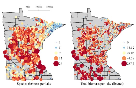
The above tables illustrate the value of the information that can be obtained using data mining techniques in R, even though most anglers are already aware of the best fishing lakes in Minnesota. A more comprehensive assessment of the data on Lakefinder is shown below. The fist two figures show species richness and total biomass (lbs per net) for the approximate 4000 lakes with fish surveys. Total biomass for each lake was the summation of the product of average weight per fish and fish per net for all species using gill net data. Total biomass can be considered a measure of lake productivity, although in many cases, this value is likely determined by a single species with high abundance (e.g., carp or bullhead).
The next two figures show average species richness and total biomass for each county. Individual values for each county are indicated.
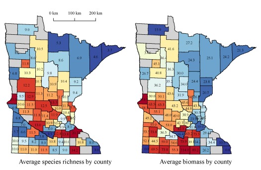
We see some pretty interesting patterns when we look at the statewide data. In general, species richness and biomass decreases along a southwest to northeast direction. These patterns vary in relation to the trophic state or productivity of each lake. We can also develop some interesting ecological hypotheses for the observed relationships. The more important implication for R users is that we’ve gathered and summarized piles of data from publicly available sources, data which can generate insight into causation. Interestingly, the maps were generated in R using the proprietary shapefile format created for ArcMap. The more I explore the packages in R that work with spatial data (e.g., sp, raster, maptools), the less I have worked with ArcMap. I’ve gone to great lengths to convince myself that the application of data mining tools available in R provide a superior alternative to commercial software. I hope that these simple examples have convinced you as well.
You can access version 2 of the catch function with the above code via my Github account. I’ve provided the following code to illustrate how the maps were produced. The data for creating the maps are not provided because this information can be obtained using the examples in this blog.
##
#first figure, summary of species richness and biomass for ~4000 lakes

require(raster)
require(sp)
require(maptools)
require(RColorBrewer) #for color ramps
require(scales) #for scaling points

par(mfrow=c(1,2),mar=numeric(4),family='serif')

#species richness
plot(counties,col='lightgrey') #get county shapefile from DNR data deli, link in blog

col.fun<-colorRampPalette(brewer.pal(11,'RdYlBu'))
col.pts<-rev(col.fun(nrow(lake.pts)))[rank(lake.pts$spp_rich)] #lake.pts can be created using 'catch.fun.v2'
rsc.pts<-rescale(lake.pts$spp_rich,c(0.5,5))
points(lake.pts$UTM_X,lake.pts$UTM_Y,cex=rsc.pts,col=col.pts,pch=19)
title(sub='Species richness per lake',line=-2,cex.sub=1.5)

leg.text<-as.numeric(summary(lake.pts$spp_rich))[-4]
leg.cex<-seq(0.5,5,length=5)
leg.col<-rev(col.fun(5))
legend(650000,5250000,legend=leg.text,pt.cex=leg.cex,col=leg.col,
       title='',pch=19,bty='n', cex=1.4,y.intersp=1.4,inset=0.11)

#scale bar
axis(side=3,
     at=c(420000,520000,620000),
     line=-4,labels=c('0 km','100 km','200 km'),
     cex.axis=1
  )

#total biomass
plot(counties,col='lightgrey')

col.fun<-colorRampPalette(brewer.pal(11,'RdYlBu'))
col.pts<-rev(col.fun(nrow(lake.pts)))[rank(lake.pts$ave.bio)]
rsc.pts<-rescale(lake.pts$ave.bio,c(0.5,5))
points(lake.pts$UTM_X,lake.pts$UTM_Y,cex=rsc.pts,col=col.pts,pch=19)
title(sub='Total biomass per lake (lbs/net)',line=-2,cex.sub=1.5)

leg.text<-as.numeric(summary(lake.pts$ave.bio))[-4]
leg.cex<-seq(0.5,5,length=5)
leg.col<-rev(col.fun(5))
legend(650000,5250000,legend=leg.text,pt.cex=leg.cex,col=leg.col,
       title='',pch=19,bty='n', cex=1.4,y.intersp=1.4,inset=0.11)

##
#second figure, county summaries

lake.pts.sp<-lake.pts #data from combination of lake polygon shapefile and catch data from catch.fun.v2
coordinates(lake.pts.sp)<-cbind(lake.pts.sp$UTM_X,lake.pts.sp$UTM_Y)

test<-over(counties,lake.pts.sp[,c(7,10)],fn=mean) #critical function for summarizing county data

co.rich<-test[,'spp_rich']
co.bio<-test[,'ave.bio']

my.cols<-function(val.in){
  pal<-colorRampPalette(brewer.pal(11,'RdYlBu')) #create color vector
  out<-numeric(length(val.in))
  out[!is.na(val.in)]<-rev(pal(sum(!is.na(val.in))))[rank(val.in[!is.na(val.in)])]
  out[out=='0']<-'lightgrey'
  out
}

#make plots
par(mfrow=c(1,2),mar=numeric(4),family='serif')
plot(counties,col=my.cols(co.rich))
text.coor<-coordinates(counties)[!is.na(co.rich),]
text(text.coor[,1],text.coor[,2],format(co.rich[!is.na(co.rich)],nsmall=1,
     digits=1),cex=0.8)
axis(side=3,
     at=c(420000,520000,620000),
     line=-4,labels=c('0 km','100 km','200 km'),
     cex.axis=1
)
title(sub='Average species richness by county',line=-2,cex.sub=1.5)

plot(counties,col=my.cols(co.bio))
text.coor<-coordinates(counties)[!is.na(co.bio),]
text(text.coor[,1],text.coor[,2],format(co.bio[!is.na(co.bio)],nsmall=1,
     digits=1),cex=0.8)
title(sub='Average biomass by county',line=-2,cex.sub=1.5)
Update: I’ve updated the catch function to return survey dates.

 for variable
  is the reciprocal of the inverse of
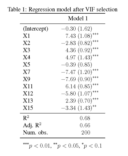
  from the regression. A VIF is calculated for each explanatory variable and those with high values are removed. The definition of ‘high’ is somewhat arbitrary but values in the range of 5-10 are commonly used.
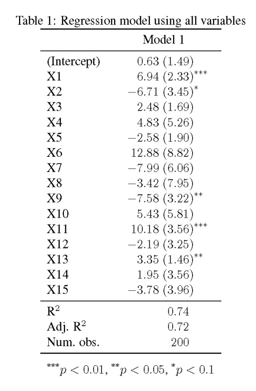
 ), yet we know that every one of the variables is related to y. As we’ll see later, the standard errors are also quite large.