
If you’re a regular reader of my blog you’ll know that I’ve spent some time dabbling with neural networks. As I explained here, I’ve used neural networks in my own research to develop inference into causation. Neural networks fall under two general categories that describe their intended use. Supervised neural networks (e.g., multilayer feed-forward networks) are generally used for prediction, whereas unsupervised networks (e.g., Kohonen self-organizing maps) are used for pattern recognition. This categorization partially describes the role of the analyst during model development. For example, a supervised network is developed from a set of known variables and the end goal of the model is to match the predicted output values with the observed via ‘supervision’ of the training process by the analyst. Development of unsupervised networks are conducted independently from the analyst in the sense that the end product is not known and no direct supervision is required to ensure expected or known results are obtained. Although my research objectives were not concerned specifically with prediction, I’ve focused entirely on supervised networks given the number of tools that have been developed to gain insight into causation. Most of these tools have been described in the primary literature but are not available in R.
My previous post on neural networks described a plotting function that can be used to visually interpret a neural network. Variables in the layers are labelled, in addition to coloring and thickening of weights between the layers. A general goal of statistical modelling is to identify the relative importance of explanatory variables for their relation to one or more response variables. The plotting function is used to portray the neural network in this manner, or more specifically, it plots the neural network as a neural interpretation diagram (NID)1. The rationale for use of an NID is to provide insight into variable importance by visually examining the weights between the layers. For example, input (explanatory) variables that have strong positive associations with response variables are expected to have many thick black connections between the layers. This qualitative interpretation can be very challenging for large models, particularly if the sign of the weights switches after passing the hidden layer. I have found the NID to be quite useless for anything but the simplest models.
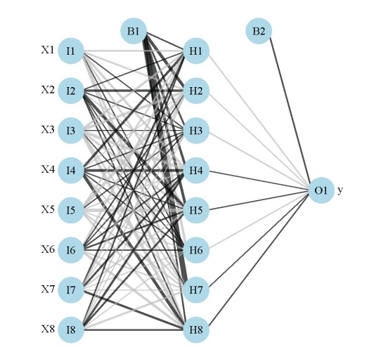
The weights that connect variables in a neural network are partially analogous to parameter coefficients in a standard regression model and can be used to describe relationships between variables. That is, the weights dictate the relative influence of information that is processed in the network such that input variables that are not relevant in their correlation with a response variable are suppressed by the weights. The opposite effect is seen for weights assigned to explanatory variables that have strong, positive associations with a response variable. An obvious difference between a neural network and a regression model is that the number of weights is excessive in the former case. This characteristic is advantageous in that it makes neural networks very flexible for modeling non-linear functions with multiple interactions, although interpretation of the effects of specific variables is of course challenging.
A method proposed by Garson 19912 (also Goh 19953) identifies the relative importance of explanatory variables for specific response variables in a supervised neural network by deconstructing the model weights. The basic idea is that the relative importance (or strength of association) of a specific explanatory variable for a specific response variable can be determined by identifying all weighted connections between the nodes of interest. That is, all weights connecting the specific input node that pass through the hidden layer to the specific response variable are identified. This is repeated for all other explanatory variables until the analyst has a list of all weights that are specific to each input variable. The connections are tallied for each input node and scaled relative to all other inputs. A single value is obtained for each explanatory variable that describes the relationship with response variable in the model (see the appendix in Goh 1995 for a more detailed description). The original algorithm presented in Garson 1991 indicated relative importance as the absolute magnitude from zero to one such the direction of the response could not be determined. I modified the approach to preserve the sign, as you’ll see below.
We start by creating a neural network model (using the nnet package) from simulated data before illustrating use of the algorithm. The model is created from eight input variables, one response variable, 10000 observations, and an arbitrary correlation matrix that describes relationships between the explanatory variables. A set of randomly chosen parameters describe the relationship of the response variable with the explanatory variables.
require(clusterGeneration)
require(nnet)

#define number of variables and observations
set.seed(2)
num.vars<-8
num.obs<-10000

#define correlation matrix for explanatory variables
#define actual parameter values
cov.mat<-genPositiveDefMat(num.vars,covMethod=c("unifcorrmat"))$Sigma
rand.vars<-mvrnorm(num.obs,rep(0,num.vars),Sigma=cov.mat)
parms<-runif(num.vars,-10,10)
y<-rand.vars %*% matrix(parms) + rnorm(num.obs,sd=20)

#prep data and create neural network
y<-data.frame((y-min(y))/(max(y)-min(y)))
names(y)<-'y'
rand.vars<-data.frame(rand.vars)
mod1<-nnet(rand.vars,y,size=8,linout=T)
The function for determining relative importance is called gar.fun and can be imported from my Github account (gist 6206737). The function reverse depends on the plot.nnet function to get the model weights.
#import 'gar.fun' from Github
source_url('https://gist.githubusercontent.com/fawda123/6206737/raw/d6f365c283a8cae23fb20892dc223bc5764d50c7/gar_fun.r')
The function is very simple to implement and has the following arguments:
out.var |
character string indicating name of response variable in the neural network object to be evaluated, only one input is allowed for models with multivariate response |
mod.in |
model object for input created from nnet function |
bar.plot |
logical value indicating if a figure is also created in the output, default T |
x.names |
character string indicating alternative names to be used for explanatory variables in the figure, default is taken from mod.in |
... |
additional arguments passed to the bar plot function |
The function returns a list with three elements, the most important of which is the last element named rel.imp. This element indicates the relative importance of each input variable for the named response variable as a value from -1 to 1. From these data, we can get an idea of what the neural network is telling us about the specific importance of each explanatory for the response variable. Here’s the function in action:
#create a pretty color vector for the bar plot
cols<-colorRampPalette(c('lightgreen','lightblue'))(num.vars)

#use the function on the model created above
par(mar=c(3,4,1,1),family='serif')
gar.fun('y',mod1,col=cols,ylab='Rel. importance',ylim=c(-1,1))

#output of the third element looks like this
# $rel.imp
#         X1         X2         X3         X4         X5
#  0.0000000  0.9299522  0.6114887 -0.9699019 -1.0000000
#         X6         X7         X8
# -0.8217887  0.3600374  0.4018899
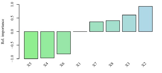
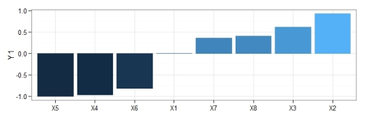
y using the neural network created above. Relative importance was determined using methods in Garson 19912 and Goh 19953. The function can be obtained here.The output from the function and the bar plot tells us that the variables X5 and X2 have the strongest negative and positive relationships, respectively, with the response variable. Similarly, variables that have relative importance close to zero, such as X1, do not have any substantial importance for y. Note that these values indicate relative importance such that a variable with a value of zero will most likely have some marginal effect on the response variable, but its effect is irrelevant in the context of the other explanatory variables.
An obvious question of concern is whether these indications of relative importance provide similar information as the true relationships between the variables we’ve defined above. Specifically, we created the response variable y as a linear function of the explanatory variables based on a set of randomly chosen parameters (parms). A graphical comparison of the indications of relative importance with the true parameter values is as follows:
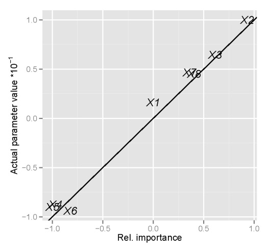
y compared to the true parameter values defined above. Parameter values were divided by ten to facilitate comparison.We assume that concordance between the true parameter values and the indications of relative importance is indicated by similarity between the two, which is exactly what is seen above. We can say with certainty that the neural network model and the function to determine relative importance is providing us with reliable information. A logical question to ask next is whether or not using a neural network provides more insight into variable relationships than a standard regression model, since we know our response variable follows the general form of a linear regression. An interesting exercise could compare this information for a response variable that is more complex than the one we’ve created above, e.g., add quadratic terms, interactions, etc.
As far as I know, Garson’s algorithm has never been modified to preserve the sign of the relationship between variables. This information is clearly more useful than simply examining the magnitude of the relationship, as is the case with the original algorithm. I hope the modified algorithm will be useful for facilitating the use of neural networks to infer causation, although it must be acknowledged that a neural network is ultimately based on correlation and methods that are more heavily based in theory could be more appropriate. Lastly, I consider this blog my contribution to dispelling the myth that neural networks are black boxes (motivated by Olden and Jackson 20024). Useful information can indeed be obtained with the right tools.
-Marcus
1Özesmi, S.L., Özesmi, U. 1999. An artificial neural network approach to spatial habitat modeling with interspecific interaction. Ecological Modelling. 116:15-31.
2Garson, G.D. 1991. Interpreting neural network connection weights. Artificial Intelligence Expert. 6(4):46–51.
3Goh, A.T.C. 1995. Back-propagation neural networks for modeling complex systems. Artificial Intelligence in Engineering. 9(3):143–151.
4Olden, J.D., Jackson, D.A. 2002. Illuminating the ‘black-box’: a randomization approach for understanding variable contributions in artificial neural networks. Ecological Modelling. 154:135-150.
Update:
I’m currently updating all of the neural network functions on my blog to make them compatible with all neural network packages in R. Additionally, the functions will be able to use raw weight vectors as inputs, in addition to model objects as currently implemented. The updates to the gar.fun function include these options. See the examples below for more details. I’ve also changed the plotting to use ggplot2 graphics.
The new arguments for gar.fun are as follows:
out.var |
character string indicating name of response variable in the neural network object to be evaluated, only one input is allowed for models with multivariate response, must be of form ‘Y1’, ‘Y2’, etc. if using numeric values as weight inputs for mod.in |
mod.in |
model object for neural network created using the nnet, RSNNS, or neuralnet packages, alternatively, a numeric vector specifying model weights in specific order, see example |
bar.plot |
logical value indicating if a figure or relative importance values are returned, default T |
struct |
numeric vector of length three indicating structure of the neural network, e.g., 2, 2, 1 for two inputs, two hidden, and one response, only required if mod.in is a vector input |
x.lab |
character string indicating alternative names to be used for explanatory variables in the figure, default is taken from mod.in |
y.lab |
character string indicating alternative names to be used for response variable in the figure, default is taken from out.var |
wts.only |
logical indicating of only model weights should be returned |
# this example shows use of raw input vector as input
# the weights are taken from the nnet model above

# import new function
source_url('https://gist.githubusercontent.com/fawda123/6206737/raw/d6f365c283a8cae23fb20892dc223bc5764d50c7/gar_fun.r')

# get vector of weights from mod1
vals.only <- unlist(gar.fun('y', mod1, wts.only = T))
vals.only
# hidden 1 11   hidden 1 12   hidden 1 13   hidden 1 14   hidden 1 15   hidden 1 16   hidden 1 17
# -1.5440440353  0.4894971240 -0.7846655620 -0.4554819870  2.3803629827  0.4045390778  1.1631255990
# hidden 1 18   hidden 1 19   hidden 1 21   hidden 1 22   hidden 1 23   hidden 1 24   hidden 1 25
# 1.5844070803 -0.4221806079  0.0480375217 -0.3983876761 -0.6046451652 -0.0736146356  0.2176405974
# hidden 1 26   hidden 1 27   hidden 1 28   hidden 1 29   hidden 1 31   hidden 1 32   hidden 1 33
# -0.0906340785  0.1633912108 -0.1206766987 -0.6528977864  1.2255953817 -0.7707485396 -1.0063172490
# hidden 1 34   hidden 1 35   hidden 1 36   hidden 1 37   hidden 1 38   hidden 1 39   hidden 1 41
# 0.0371724519  0.2494350900  0.0220121908 -1.3147089165  0.5753711352  0.0482957709 -0.3368124708
# hidden 1 42   hidden 1 43   hidden 1 44   hidden 1 45   hidden 1 46   hidden 1 47   hidden 1 48
# 0.1253738473  0.0187610286 -0.0612728942  0.0300645103  0.1263138065  0.1542115281 -0.0350399176
# hidden 1 49   hidden 1 51   hidden 1 52   hidden 1 53   hidden 1 54   hidden 1 55   hidden 1 56
# 0.1966119466 -2.7614366991 -0.9671345937 -0.1508876798 -0.2839796515 -0.8379801306  1.0411094014
# hidden 1 57   hidden 1 58   hidden 1 59   hidden 1 61   hidden 1 62   hidden 1 63   hidden 1 64
# 0.7940494280 -2.6602412144  0.7581558506 -0.2997650961  0.4076177409  0.7755417212 -0.2934247464
# hidden 1 65   hidden 1 66   hidden 1 67   hidden 1 68   hidden 1 69   hidden 1 71   hidden 1 72
# 0.0424664179  0.5997626459 -0.3753986118 -0.0021020946  0.2722725781 -0.2353500011  0.0876374693
# hidden 1 73   hidden 1 74   hidden 1 75   hidden 1 76   hidden 1 77   hidden 1 78   hidden 1 79
# -0.0244290095 -0.0026191346  0.0080349427  0.0449513273  0.1577298156 -0.0153099721  0.1960918520
# hidden 1 81   hidden 1 82   hidden 1 83   hidden 1 84   hidden 1 85   hidden 1 86   hidden 1 87
# -0.6892926134 -1.7825068475  1.6225034225 -0.4844547498  0.8954479895  1.1236485983  2.1201674117
# hidden 1 88   hidden 1 89        out 11        out 12        out 13        out 14        out 15
# -0.4196627413  0.4196025359  1.1000994866 -0.0009401206 -0.3623747323  0.0011638613  0.9642290448
# out 16        out 17        out 18        out 19
# 0.0005194378 -0.2682687768 -1.6300590889  0.0021911807

# use the function and modify ggplot object
p1 <- gar.fun('Y1',vals.only, struct = c(8,8,1))
p1

p2 <- p1 + theme_bw() + theme(legend.position = 'none')
p2
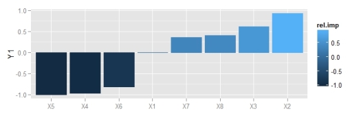
ggplot2 theme.
The user has the responsibility to make sure the weight vector is in the correct order if raw weights are used as input. The function will work if all weights are provided but there is no method for identifying the correct order. The names of the weights in the commented code above describe the correct order, e.g., Hidden 1 11 is the bias layer weight going to hidden node 1, Hidden 1 12 is the first input going to the first hidden node, etc. The first number is an arbitrary place holder indicating the first hidden layer. The correct structure must also be provided for the given length of the input weight vector. NA values should be used if no bias layers are included in the model. Stay tuned for more updates as I continue revising these functions.
