I’ve just released an updated version of my package for estuary monitoring data, SWMPr, available on CRAN. I’ve made several additions to the package since it’s initial release – nothing too crazy but enough to warrant another push to CRAN and blog post. I’ve been pretty bad about regular updates but I’ve added a few features to make some of the functions easier to use in addition to some new functions for plotting SWMP data. I’ll start with a brief overview of the package then describe some of the major changes since the last release (2.0.0). As always, please keep a close watch on the GitHub repository for progress on the development version of the package.
What is SWMPr? SWMPr is an R package for estuary monitoring data from the National Estuarine Research Reserve System (NERRS). NERRS is a collection of reserve programs located at 28 estuaries in the United States. The System-Wide Monitoring Program (SWMP) was established by NERRS in 1995 as a long-term monitoring program to collect water quality, nutrient, and weather data at over 140 stations (more info here). To date, over 58 million records have been collected and are available online through the Centralized Data Management Office (CDMO). The SWMPr package provides a bridge between R and the data provided by SWMP (which explains the super clever name). The package is meant to augment existing CDMO services and to provide more generic features for working with water quality time series. The initial release included functions to import SWMP data from the CDMO directly into R, functions for data organization, and some basic analysis functions. The original release also included functions for estimating rates of ecosystem primary production using the open-water method.
# installing and loading the package
install.packages('SWMPr')
library(SWMPr)
What’s new in 2.1? A full list of everything that’s changed can be viewed here. Not all these changes are interesting (bugs mostly), but they are worth viewing if you care about the nitty gritty. The most noteworthy changes include the following.
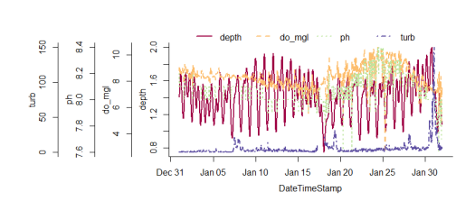
The overplot function can be used to plot multiple variables with identical scaling on the y-axis. I think this is generally discouraged under sound plotting theory (see the rants here), but overplotting is an often-requested feature regardless of popular opinion. I had to use the base graphics to write this function since it’s not possible with ggplot. I actually borrowed most of the code from a colleague at NERRS, shouts to the Grand Bay office. To illustrate ease of use…
# import data and do some initial clean up
data(apacpwq)
dat <- qaqc(apacpwq)

# a truly heinous plot
overplot(dat, select = c('depth', 'do_mgl', 'ph', 'turb'),
  subset = c('2013-01-01 0:0', '2013-02-01 0:0'), lwd = 2)
The qaqc function now has more flexible filtering of QAQC data flags by using regular expression matching, rather than searching by integer flags as in the previous version. What this means is that observations can be filtered with greater control over what flags and errors are removed. This example shows how to remove flags using the old method as integer flags and using the new method. The second example will keep all flags that are annotated with the ‘CSM’ comment code (meaning check the metadata). The value with this approach is that not all integer flags are coded the same, i.e., QAQC flags with the same integer may not always have the same error code. The user may not want to remove all flags of a single type if only certain error codes are important.
# import data
data(apadbwq)
dat <- apadbwq

# retain only '0' and '-1' flags, as in the older version
newdat <- qaqc(dat, qaqc_keep = c('0', '-1'))

# retain observations with the 'CSM' error code
newdat <- qaqc(dat, qaqc_keep = 'CSM')
Several of the data import functions were limited in the total number of records that could be requested from the CDMO. I made some dirty looping hacks so that most of these rate limitations, although technically still imposed, can be ignored when making large data requests to the CDMO. Previously, the single_param, all_params, and all_params_dtrng functions were limited to 100 records in a single request – not very useful for time series taken every 15 minutes. The new version lets you download any number of records using these functions, although be warned that the data request can take a long time for larger requests. As before, your computer’s IP address must be registered with the CDMO to use these functions.
Although it’s now theoretically possible to retrieve all the SWMP data with the above functions, using the import_local function is still much, much easier. The main advantage of this function is that local data can be imported into R, which allows the user to import large amounts of data from a single request. The new release of SWMPr makes this process even easier by allowing data to be imported directly from the compressed, zipped data folder returned from the CDMO data request. The syntax is the same, but the full path including the .zip file extension must be included. As before, this function is designed to be used with data from the zip downloads feature of the CDMO.
# this is the path for the downloaded data files, zipped folder
path <- 'C:/this/is/my/data/path.zip'

# import the data
dat <- import_local(path, 'apaebmet')
A nice feature in R documentation that I recently discovered is the ability to search for functions by ‘concept’ or ‘alias’ tags. I’ve described the functions in SWMPr as being in one of three categories based on their intended use in the data workflow: retrieve, organize, and analyze. The new version of SWMPr uses these categories as search terms for finding the help files for each function. The package includes additional functions not in these categories but they are mostly intended as helpers for the primary functions. As always, consult the manual for full documentation.
Finally, I’ve added several default methods to existing SWMPr functions to make them easier to use outside of the normal SWMPr workflow. For example, combining time series with different time steps is a common challenge prior to data analysis. The comb function achieves this task for SWMP data, although using the previous release of the package on generic data was rather clunky. The new default method makes it easier to combine data objects with a generic format (data frames), provided a few additional arguments are provided so the function knows how to handle the information. Default methods were also added for the setstep, decomp, and decomp_cj functions.
I guarantee there are some bugs in this new release and I gladly welcome bug reports on the issues tab of the development repo. Ideas for additional features can also be posted. Please check out our SWMPrats web page for other SWMP-related analysis tools.
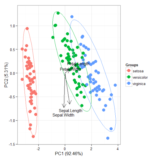
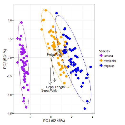
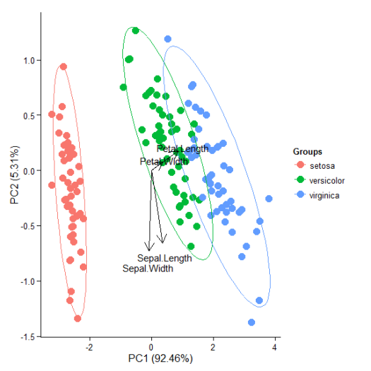
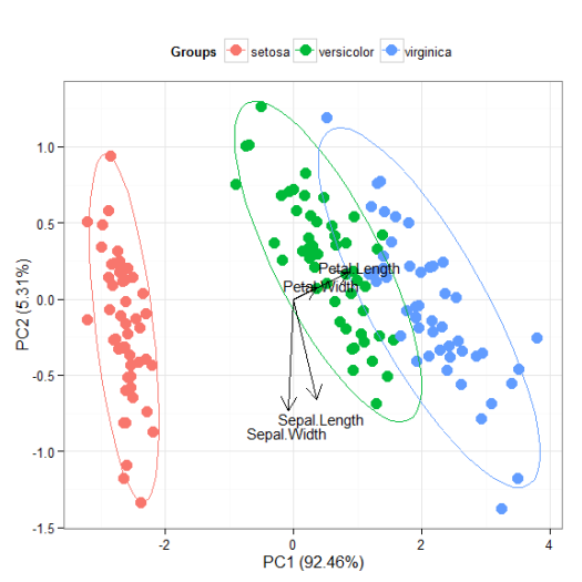
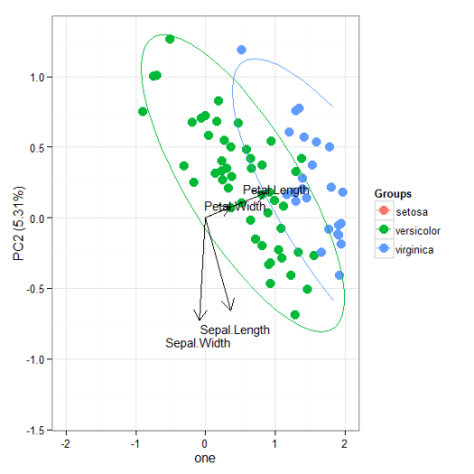
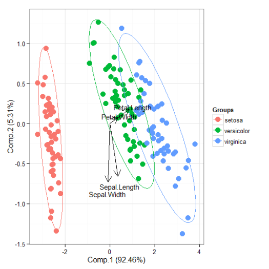
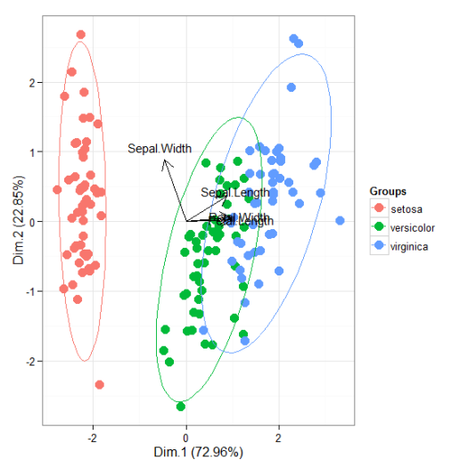
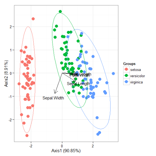
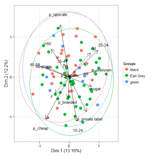
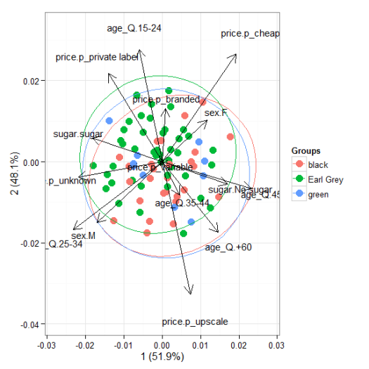
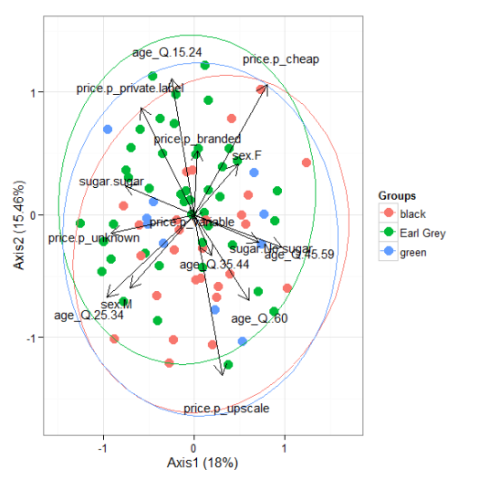
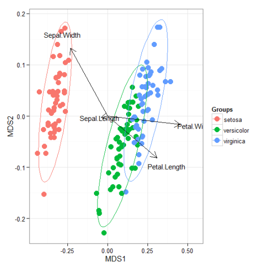
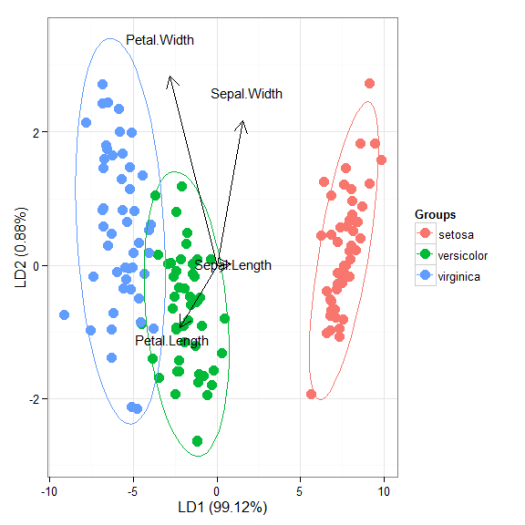
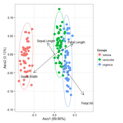
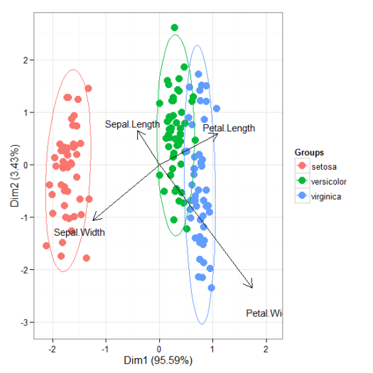
I’ll be the first to admit that the topic of plotting ordination results using ggplot2 has been visited many times over. As is my typical fashion, I started creating a package for this purpose without completely searching for existing solutions. Specifically, the ggbiplot and factoextra packages already provide almost complete coverage of plotting results from multivariate and ordination analyses in R. Being the stubborn individual, I couldn’t give up on my own package so I started exploring ways to improve some of the functionality of biplot methods in these existing packages. For example, ggbiplot and factoextra work almost exclusively with results from principal components analysis, whereas numerous other multivariate analyses can be visualized using the biplot approach. I started to write methods to create biplots for some of the more common ordination techniques, in addition to all of the functions I could find in R that conduct PCA. This exercise became very boring very quickly so I stopped adding methods after the first eight or so. That being said, I present this blog as a sinking ship that was doomed from the beginning, but I’m also hopeful that these functions can be built on by others more ambitious than myself.
The process of adding methods to a default biplot function in ggplot was pretty simple and not the least bit interesting. The default ggpord biplot function (see here) is very similar to the default biplot function from the stats base package. Only two inputs are used, the first being a two column matrix of the observation scores for each axis in the biplot and the second being a two column matrix of the variable scores for each axis. Adding S3 methods to the generic function required extracting the relevant elements from each model object and then passing them to the default function. Easy as pie but boring as hell.
I’ll repeat myself again. This package adds nothing new to the functionality already provided by ggbiplot and factoextra. However, I like to think that I contributed at least a little bit by adding more methods to the biplot function. On top of that, I’m also naively hopeful that others will be inspired to fork my package and add methods. Here you can view the raw code for the ggord default function and all methods added to that function. Adding more methods is straightforward, but I personally don’t have any interest in doing this myself. So who wants to help??
Visit the package repo here or install the package as follows.
I’m pleased to announce that my second R package, SWMPr, has been posted on CRAN. I developed this package to work with water quality time series data from the System Wide Monitoring Program (SWMP) of the National Estuarine Research Reserve System (NERRS). SWMP was established in 1995 to provide continuous environmental data at over 300 fixed stations in 28 estuaries of the United States (more info here). SWMP data are collected with the general objective of describing dynamics of estuarine ecosystems to better inform coastal management. However, simple tools for processing and evaluating the increasing quantity of data provided by the monitoring network have complicated broad-scale comparisons between systems and, in some cases, simple trend analysis of water quality parameters at individual sites. The SWMPr package was developed to address common challenges of working with SWMP data by providing functions to retrieve, organize, and analyze environmental time series data.
The development version of this package lives on GitHub. It can be installed from CRAN and loaded in R as follows:
install.packages('SWMPr')
library(SWMPr)
SWMP data are maintained online by the Centralized Data Management Office (CDMO). Time series data describing water quality, nutrient, or weather observations can be downloaded for any of the 28 estuaries. Several functions are provided by the SWMPr package that allow import of data from CDMO into R, either through direct download through the existing web services or by local (import_local) or remote (import_remote) sources. Imported data are loaded as swmpr objects with several attributes following standard S3 object methods. The remaining functions in the package are used to organize and analyze the data using a mix of standard methods for time series and more specific approaches developed for SWMP. This blog concludes with a brief summary of the available functions, organized by category. As always, be sure to consult the help documentation for more detailed information.
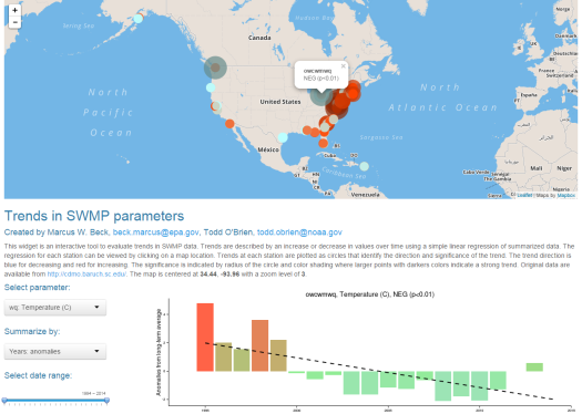
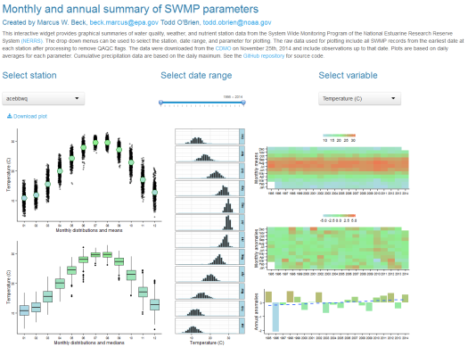
I’ve also created two shiny applications to illustrate the functionality provided by the package. The first shiny app evaluates trends in SWMP data within and between sites using an interactive map. Trends between reserves can be viewed using the map, whereas trends at individual sites can be viewed by clicking on a map location. The data presented on the map were imported and processed using the import_local, qaqc, and aggregate functions. The second app provides graphical summaries of water quality, weather, or nutrient data at individual stations using the plot_summary function. Data were also processed with the import_local, qaqc, and aggregate functions.
SWMP trends map (click to access):
SWMP summary map (click to access):
SWMPr functions
Below is a brief description of each function in the SWMPr package. I’m currently working on a manuscript to describe use of the package in much greater detail. For now, please visit our website that introduced version 1.0.0 of the SWMPr package (check the modules tab).
Retrieve
all_params
Retrieve up to 100 records starting with the most recent at a given station, all parameters. Wrapper to exportAllParamsXMLNew function on web services.
all_params_dtrng
Retrieve records of all parameters within a given date range for a station. Optional argument for a single parameter. Maximum of 1000 records. Wrapper to exportAllParamsDateRangeXMLNew.
import_local
Import files from a local path. The files must be in a specific format, specifically those returned from the CDMO using the zip downloads option for a reserve.
import_remote
Import SWMP site data from a remote independent server. These files have been downloaded from CDMO, processed using functions in this package, and uploaded to an Amazon server for quicker import into R.
single_param
Retrieve up to 100 records for a single parameter starting with the most recent at a given station. Wrapper to exportSingleParamXMLNew function on web services.
Organize
comb.swmpr
Combines swmpr objects to a common time series using setstep, such as combining the weather, nutrients, and water quality data for a single station. Only different data types can be combined.
qaqc.swmpr
Remove QAQC columns and remove data based on QAQC flag values for a swmpr object. Only applies if QAQC columns are present.
qaqcchk.swmpr
View a summary of the number of observations in a swmpr object that are assigned to different QAQC flags used by CDMO. The output is used to inform further processing but is not used explicitly.
rem_reps.swmpr
Remove replicate nutrient data that occur on the same day. The default is to average replicates.
setstep.swmpr
Format data from a swmpr object to a continuous time series at a given timestep. The function is used in comb.swmpr and can also be used with individual stations.
subset.swmpr
Subset by dates and/or columns for a swmpr object. This is a method passed to the generic `subset’ function provided in the base package.
Analyze
aggreswmp.swmpr
Aggregate swmpr objects for different time periods – years, quarters, months, weeks, days, or hours. Aggregation function is user-supplied but defaults to mean.
aggremetab.swmpr
Aggregate metabolism data from a swmpr object. This is primarily used within plot_metab but may be useful for simple summaries of raw daily data.
ecometab.swmpr
Estimate ecosystem metabolism for a combined water quality and weather dataset using the open-water method.
decomp.swmpr
Decompose a swmpr time series into trend, seasonal, and residual components. This is a simple wrapper to decompose. Decomposition of monthly or daily trends is possible.
decomp_cj.swmpr
Decompose a swmpr time series into grandmean, annual, seasonal, and events components. This is a simple wrapper to decompTs in the wq package. Only monthly decomposition is possible.
hist.swmpr
Plot a histogram for a swmpr object.
lines.swmpr
Add lines to an existing swmpr plot.
na.approx.swmpr
Linearly interpolate missing data (NA values) in a swmpr object. The maximum gap size that is interpolated is defined as a maximum number of records with missing data.
plot.swmpr
Plot a univariate time series for a swmpr object. The parameter name must be specified.
plot_metab
Plot ecosystem metabolism estimates after running ecometab on a swmpr object.
plot_summary
Create summary plots of seasonal/annual trends and anomalies for a water quality or weather parameter.
smoother.swmpr
Smooth swmpr objects with a moving window average. Window size and sides can be specified, passed to filter.
Miscellaneous
calcKL
Estimate the reaeration coefficient for air-sea gas exchange. This is only used within the ecometab function.
map_reserve
Create a map of all stations in a reserve using the ggmap package.
metab_day
Identify the metabolic day for each approximate 24 period in an hourly time series. This is only used within the ecometab function.
param_names
Returns column names as a list for the parameter type(s) (nutrients, weather, or water quality). Includes QAQC columns with ‘f_’ prefix. Used internally in other functions.
parser
Parses html returned from CDMO web services, used internally in retrieval functions.
site_codes
Metadata for all stations, wrapper to exportStationCodesXMLNew function on web services.
site_codes_ind
Metadata for all stations at a single site, wrapper to NERRFilterStationCodesXMLNew function on web services.
swmpr
Creates object of swmpr class, used internally in retrieval functions.
time_vec
Converts time vectors to POSIX objects with correct time zone for a site/station, used internally in retrieval functions.
After successfully navigating the perilous path of CRAN submission, I’m pleased to announce that NeuralNetTools is now available! From the description file, the package provides visualization and analysis tools to aid in the interpretation of neural networks, including functions for plotting, variable importance, and sensitivity analyses. I’ve written at length about each of these functions (see here, here, and here), so I’ll only provide an overview in this post. Most of these functions have remained unchanged since I initially described them, with one important change for the Garson function. Rather than reporting variable importance as -1 to 1 for each variable, I’ve returned to the original method that reports importance as 0 to 1. I was getting inconsistent results after toying around with some additional examples and decided the original method was a safer approach for the package. The modified version can still be installed from my GitHub gist. The development version of the package is also available on GitHub. Please use the development page to report issues.
The package is fairly small but I think the functions that have been included can help immensely in evaluating neural network results. The main functions include:
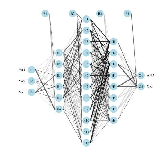
plotnet: Plot a neural interpretation diagram for a neural network object, original blog post here
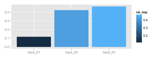
garson: Relative importance of input variables in neural networks using Garson’s algorithm, original blog post here
# create model
library(RSNNS)
data(neuraldat)
x <- neuraldat[, c('X1', 'X2', 'X3')]
y <- neuraldat[, 'Y1']
mod <- mlp(x, y, size = 5)

# garson
garson(mod, 'Y1')
Fig: Using the garson function.
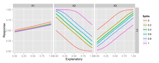
lekprofile: Conduct a sensitivity analysis of model responses in a neural network to input variables using Lek’s profile method, original blog post here
# create model
library(nnet)
data(neuraldat)
mod <- nnet(Y1 ~ X1 + X2 + X3, data = neuraldat, size = 5)

# lekprofile
lekprofile(mod)
Fig: Using the lekprofile function.
A few other functions are available that are helpers to the main functions. See the documentation for a full list.
All the functions have S3 methods for most of the neural network classes available in R, making them quite flexible. This includes methods for nnet models from the nnet package, mlp models from the RSNNS package, nn models from the neuralnet package, and train models from the caret package. The functions also have methods for numeric vectors if the user prefers inputting raw weight vectors for each function, as for neural network models created outside of R.
Huge thanks to Hadley Wickham for his packages that have helped immensely with this process, namely devtools and roxygen2. I also relied extensively on his new web book for package development. Any feedback regarding NeuralNetTools or its further development is appreciated!
I remember my first experience installing R. Basic installation can be humbling for someone not familiar with mirror networks or file binaries. I remember not knowing the difference between base and contrib… which one to select? The concept of CRAN and mirrors was also new to me. Which location do I choose and are they all the same? What the hell is a tar ball?? Simple challenges like these can be discouraging to first-time users that have never experienced the world of open-source software. Although these challenges seem silly now, they were very real at the time. Additionally, help documentation is not readily accessible for the novice. This month I decided to step back and present a simple guide to installing R and RStudio. Surprisingly, a quick Google search was unable to locate comparable guides. I realize that most people don’t have any problem installing R, but I can remember a time when step-by-step installation instructions would have been very appreciated. Also, I made this guide for a workshop and I’m presenting it here so I don’t have to create a different blog post for this month… I am lazy. Files for creating the guide are available here.
With all the recent buzz about ggvis (this, this, and this) it’s often easy to forget all that ggplot2 offers as a graphics package. True, ggplot is a static approach to graphing unlike ggvis but it has fundamentally changed the way we think about plots in R. I recently spent some time thinking about some of the more useful features of ggplot2 to answer the question ‘what is offered by ggplot2 that one can’t do with the base graphics functions?’ First-time users of ggplot2 are often confused by the syntax, yet it is precisely this syntax built on the philosophy of the grammar of graphics that makes ggplot2 so powerful. Adding content layers to mapped objects are central to this idea, which allows linking of map aesthetics through a logical framework. Additionally, several packages have been developed around this philosophy to extend the functionality of ggplot2 in alternative applications (e.g., ggmap, GGally, ggthemes).
I recently gave a presentation to describe some of my favorite features of ggplot2 and other packages building on its core concepts. I describe the use of facets for multi-panel plots, default and custom themes, ggmap for spatial mapping with ggplot2, and GGally for generalized pairs plots. Although this is certainly a subjective and incomplete list, my workflows have become much more efficient (and enjoyable) by using these tools. Below is a link to the presentation. Note that this will not load using internet explorer and you may have to reload if using Chrome to get the complete slide deck. This is my first time hosting a Slidify presentation on RPubs, so please bear with me. The presentation materials are also available at Github.
.
What are some of your favorite features of ggplot2??
The challenge of integrating Microsoft products with R software has been an outstanding issue for several years. Reasons for these issues are complicated and related to fundamental differences in developing proprietary vs open-source products. To date, I don’t believe there has been a satisfactory solution but I present this blog as my attempt to work around at least some of the issues using the two. As a regular contributor to R-bloggers, I stress that one should use MS products as little as possible given the many issues that have been described (for example, here, here, and here). It’s not my intent to pick on Microsoft. In fact, I think Excel is a rather nifty program that has its place in specific situations. However, most of my work is not conducive to the point-and-click style of spreadsheet analysis and the surprising limited number of operations available in Excel prevent all but the simplest analyses. I try my best to keep my work within the confines of RStudio, given its integration with multiple document preparation systems.
I work with several talented researchers that have different philosophies than my own on the use of Microsoft products. It’s inevitable that we’re occasionally at odds. Our difficulties go both directions — my insistence on using pdfs for creating reports or manuscripts and the other party’s inclination towards the spreadsheet style of analysis. It seems silly that we’re limited by the types of medium we prefer. I’ve recently been interested in developing a workflow that addresses some of the issues of using end-products from different sources under the notion of reproducibility. To this end, I used Pandoc and relevant R packages (namely gdata and knitr) to develop a stand-alone workflow that allows integration of Microsoft products with my existing workflows. The idea is simple. I want to import data sent to me in .xlsx format, conduct the analysis and report generation entirely within RStudio, and convert the output to .docx format on completion. This workflow allows all tasks to be completed within RStudio, provided the supporting documents, software, and packages work correctly.
Of course, I don’t propose this workflow as a solution to all issues related to Office products and R. I present this material as a conceptual and functional design that could be used by others with similar ideas. I’m quite happy with this workflow for my personal needs, although I’m sure it could be improved upon. I describe this workflow using the pdf below and provide all supporting files on Github: https://github.com/fawda123/pan_flow.
\documentclass[xcolor=svgnames]{beamer}
\usetheme{Boadilla}
\usecolortheme[named=SeaGreen]{structure}
\usepackage{graphicx}
\usepackage{breqn}
\usepackage{xcolor}
\usepackage{booktabs}
\usepackage{verbatim}
\usepackage{tikz}
\usetikzlibrary{shadows,arrows,positioning}
\definecolor{links}{HTML}{2A1B81}
\hypersetup{colorlinks,linkcolor=links,urlcolor=links}
\usepackage{pgfpages}

\tikzstyle{block} = [rectangle, draw, text width=9em, text centered, rounded corners, minimum height=3em, minimum width=7em, top color = white, bottom color=brown!30,  drop shadow]

\newcommand{\ShowSexpr}[1]{\texttt{{\char`\\}Sexpr\{#1\}}}

\begin{document}

\title[R with Microsoft]{A simple workflow for using R with Microsoft products}
\author[M. Beck]{Marcus W. Beck}

\institute[USEPA NHEERL]{USEPA NHEERL Gulf Ecology Division, Gulf Breeze, FL\\
Email: \href{mailto:beck.marcus@epa.gov}{beck.marcus@epa.gov}, Phone: 850 934 2480}

\date{May 21, 2014}

%%%%%%
\begin{frame}
\vspace{-0.3in}
\titlepage
\end{frame}

%%%%%%
\begin{frame}{The problem...}
\begin{itemize}
\item R is great and has an increasing user base\\~\\
\item RStudio is integrated with multiple document preparation systems \\~\\
\item Output documents are not in a format that facilitates collaboration with
non R users, e.g., pdf, html \\~\\
\item Data coming to you may be in a proprietary format, e.g., xls spreadsheet
\end{itemize}
\end{frame}

%%%%%%
\begin{frame}{The solution?}
\begin{itemize}
\item Solution one - Make liberal use of `projects' within RStudio \\~\\
\item Solution two - Use \texttt{gdata} package to import excel data \\~\\
\item Solution three - Get pandoc to convert document formats - \href{http://johnmacfarlane.net/pandoc/}{http://johnmacfarlane.net/pandoc/} \\~\\
\end{itemize}
\onslide<2->
\large
\centerline{\textit{Not recommended for simple tasks unless you really, really love R}}
\end{frame}

%%%%%
\begin{frame}{An example workflow}
\begin{itemize}
\item I will present a workflow for integrating Microsoft products within RStudio as an approach to working with non R users \\~\\
\item Idea is to never leave the RStudio environment - dynamic documents! \\~\\
\item General workflow... \\~\\
\end{itemize}
\small
\begin{center}
\begin{tikzpicture}[node distance=2.5cm, auto, >=stealth]
  \onslide<2->{
	\node[block] (a) {1. Install necessary software and packages};}
	\onslide<3->{
	\node[block] (b)  [right of=a, node distance=4.2cm] {2. Create project in RStudio};
 	\draw[->] (a) -- (b);}
 	\onslide<4->{
 	\node[block] (c)  [right of=b, node distance=4.2cm]  {3. Setup supporting docs/functions};
 	\draw[->] (b) -- (c);}
   \onslide<5->{
   \node[block] (d)  [below of=a, node distance=2.5cm]  {4. Import with \texttt{gdata}, summarize};
 	\draw[->] (c) -- (d);}
   \onslide<6->{
   \node[block] (e)  [right of=d, node distance=4.2cm]  {5. Create HTML document using knitr Markdown};
 	\draw[->] (d) -- (e);}
     \onslide<7->{
   \node[block] (f)  [right of=e, node distance=4.2cm]  {6. Convert HTML doc to Word with Pandoc};
   \draw[->] (e) -- (f);}
\end{tikzpicture}
\end{center}
\end{frame}

%%%%%%
\begin{frame}[shrink]{The example}
You are sent an Excel file of data to summarize and report but you love R and want to do everything in RStudio...
<<echo = F, results = 'asis', message = F>>=
library(gdata)
library(xtable)

prl_pth <- 'C:/strawberry/perl/bin/perl.exe'
url <- 'https://beckmw.files.wordpress.com/2014/05/my_data.xlsx'
dat <- read.xls(xls = url, sheet = 'Sheet1', perl = prl_pth)
out.tab <- xtable(dat, digits=4)
print.xtable(out.tab, type = 'latex', include.rownames = F,
  size = 'scriptsize')
@
\end{frame}

%%%%%%
\begin{frame}{Step 1}
Install necessary software and Packages \\~\\
\onslide<1->
\begin{itemize}
\onslide<2->
\item R and RStudio (can do with other R editors)\\~\\
\item Microsoft Office\\~\\
\onslide<3->
\item Strawberry Perl for using \texttt{gdata} package\\~\\
\item Pandoc\\~\\
\onslide<4->
\item Packages: \texttt{gdata}, \texttt{knitr}, \texttt{utils}, \texttt{xtable}, others as needed...
\end{itemize}
\end{frame}

%%%%%%
\begin{frame}{Step 2}
Create a project in RStudio \\~\\
\begin{itemize}
\item Create a folder or use existing on local machine \\~\\
\item Add .Rprofile file to the folder for custom startup \\~\\
\item Move all data you are working with to the folder \\~\\
\item Literally create project in RStudio \\~\\
\item Set options within RStudio \\~\\
\end{itemize}
\end{frame}

%%%%%%
\begin{frame}[fragile]{Step 3}
Setup supporting docs/functions, i.e., .Rprofile, functions, report, master
\scriptsize
\begin{block}{.Rprofile}
<<echo = T, eval = F, results = 'markup'>>=
# library path
.libPaths('C:\\Users\\mbeck\\R\\library')

# startup message
cat('My project...\n')

# packages to use
library(utils) # for system commands
library(knitr) # for markdown
library(gdata) # for import xls
library(reshape2) # data format conversion
library(xtable) # easy tables
library(ggplot2) # plotting

# perl path for gdata
prl_pth <- 'C:/strawberry/perl/bin/perl.exe'

# functions to use
source('my_funcs.r')
@
\end{block}
\end{frame}

%%%%%%
\begin{frame}[t, fragile]{Step 3}
Setup supporting docs/functions, i.e., .Rprofile, functions, report, master
\scriptsize
\begin{block}{my\_funcs.r}
<<echo = T, eval = F, results = 'markup'>>=
######
# functions for creating report,
# created May 2014, M. Beck

######
# processes data for creating output in report,
# 'dat_in' is input data as data frame,
# output is data frame with converted variables
proc_fun<-function(dat_in){

  # convert temp to C
  dat_in$Temperature <- round((dat_in$Temperature - 32) * 5/9)

  #  convert data to long format
  dat_in <- melt(dat_in, measure.vars = c('Restoration', 'Reference'))

  return(dat_in)

}

######
# creates linear model for data,
# 'proc_dat' is processed data returned from 'proc_fun',
# output is linear model object
mod_fun <- function(proc_in) lm(value ~ variable + Year, dat = proc_in)
@
\end{block}
\end{frame}

%%%%%%
\begin{frame}[fragile,shrink]{Step 3}
Setup supporting docs/functions, i.e., .Rprofile, functions, report, master
\scriptsize
\begin{block}{report.Rmd}
\begin{verbatim}
======================
Here's a report I made for `r gsub('/|.xlsx','',name)`
----------------------

```{r echo=F, include=F}
# import data
url <- paste0('https://beckmw.files.wordpress.com/2014/05', name)
dat <- read.xls(xls = url, sheet = 'Sheet1', perl = prl_pth)

# process data for tables/figs
dat <- proc_fun(dat)

# model of data
mod <- mod_fun(dat)
```

### Model summary
```{r results='asis', echo=F}
print.xtable(xtable(mod, digits = 2), type = 'html')
```

### Figure of restoration and reference by year
```{r reg_fig, echo = F, fig.width = 5, fig.height = 3, dpi=200}
ggplot(dat, aes(x = Year, y = value, colour = variable)) +
  geom_point() +
  stat_smooth(method = 'lm')
```
\end{verbatim}
\end{block}
\end{frame}

%%%%%%
\begin{frame}[t, fragile]{Step 3}
Setup supporting docs/functions, i.e., .Rprofile, functions, report, master
\scriptsize
\begin{block}{master.r}
<<echo = T, eval = F, results = 'markup'>>=
# file to process
name <- '/my_data.xlsx'

# rmd to html
knit2html('report.Rmd')

# pandoc conversion of html to word doc
system(paste0('pandoc -o report.docx report.html'))
@
\end{block}
\end{frame}

%%%%%%
\begin{frame}[fragile]{Steps 4 - 6}
\small
After creating supporting documents in Project directory, final steps are completed by running `master.r'
\begin{itemize}
\item Step 4 - xls file imported using \texttt{gdata} package, implemented in `report.Rmd'
\item Step 5 - HTML document created by converting `report.Rmd' with \texttt{knit2html} in `master.r'
\item Step 6 - HTML document converted to Word with Pandoc by invoking system command
\end{itemize}
\begin{block}{master.r}
<<echo = T, eval = F, results = 'markup'>>=
# file to process
name <- '/my_data.xlsx'

# rmd to html
knit2html('report.Rmd')

# pandoc conversion of html to word doc
system(paste0('pandoc -o report.docx report.html'))
@
\end{block}
\end{frame}


\end{document}
To use the workflow, start a new version control project through Git in RStudio, pull the files from the repository, and run the master file. An excellent introduction for using RStudio with Github can be found here. I’ve also included two excel files that can be used to generate the reports. You can try using each one by changing the name variable in the master file and then running the commands:
name <- 'my_data.xlsx'
knit2html('report.Rmd')
system(paste0('pandoc -o report.docx report.html'))
or…
name <- 'my_data_2.xlsx'
knit2html('report.Rmd')
system(paste0('pandoc -o report.docx report.html'))
The output .docx file should be different depending on which Excel file you use as input. As the pdf describes, none of this will work if you don’t have the required software/packages, i.e., R/RStudio, Strawberry Perl, Pandoc, MS Office, knitr, gdata, etc. You’ll also need Git installed if you are pulling the files for local use (again, see here). I’d be interested to hear if anyone finds this useful or any general comments on improvements/suggestions for the workflow.
This past week I attended the National Water Quality Monitoring Conference in Cincinnati. Aside from spending my time attending talks, workshops, and meeting like-minded individuals, I spent an unhealthy amount of time in the hotel bar working on this blog post. My past experiences mixing coding and beer have suggested the two don’t mix, but I was partly successful in writing a function that will be the focus of this post.
I’ve often been curious how much code I’ve written over the years since most of my professional career has centered around using R in one form or another. In the name of ridiculous self-serving questions, I wrote a function for quantifying code lengths by file type. I would describe myself as somewhat of a hoarder with my code in that nothing ever gets deleted. Getting an idea of the total amount was a simple exercise in finding the files, enumerating the file contents, and displaying the results in a sensible manner.
I was not surprised that several functions in R already exist for searching for file paths in directory trees. The list.files function can be used to locate files using regular expression matching, whereas the file.info function can be used to get descriptive information for each file. I used both in my function to find files in a directory tree through recursive searching of paths with a given extension name. The date the files was last modified is saved, and the file length, as lines or number of characters, is saved after reading the file with readLines. The output is a data frame for each file with the file name, type, length, cumulative length by file type, and date. The results can be easily plotted, as shown below.
The function, obtained here, has the following arguments:
root
Character string of root directory to search
file_typs
Character vector of file types to search, file types must be compatible with readLines
omit_blank
Logical indicating of blank lines are counted, default TRUE
recursive
Logical indicating if all directories within root are searched, default TRUE
lns
Logical indicating if lines in each file are counted, default TRUE, otherwise characters are counted
trace
Logical for monitoring progress, default TRUE
Here’s an example using the function to search a local path on my computer.
# import function from Github
library(devtools)

# https://gist.github.com/fawda123/20688ace86604259de4e
source_gist('20688ace86604259de4e')

# path to search and file types
root <- 'C:/Projects'
file_typs <- c('r','py', 'tex', 'rnw')

# get data from function
my_fls <- file.lens(root, file_typs)

head(my_fls)

##                               fl Length       Date cum_len Type
## 1                 buffer loop.py     29 2010-08-12      29   py
## 2                  erase loop.py     22 2010-08-12      51   py
## 3 remove selection and rename.py     26 2010-08-16      77   py
## 4              composite loop.py     32 2010-08-18     109   py
## 5                extract loop.py     61 2010-08-18     170   py
## 6         classification loop.py     32 2010-08-19     202   py
In this example, I’ve searched for R, Python, LaTeX, and Sweave files in the directory ‘C:/Projects/’. The output from the function is shown using the head command.
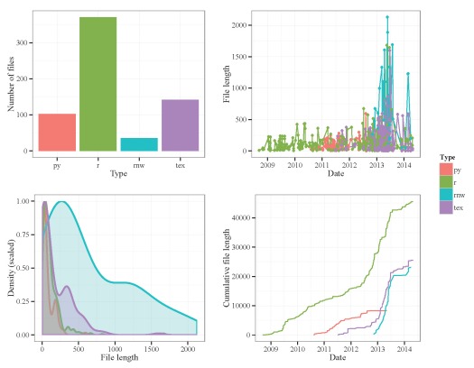
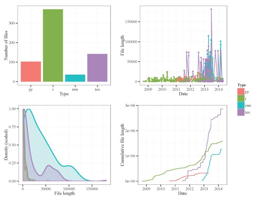
Here’s some code for plotting the data. I’ve created four plots with ggplot and combined them using grid.arrange from the gridExtra package. The first plot shows the number of files by type, the second shows file length by date and type, the third shows a frequency distribution of file lengths by type, and the fourth shows a cumulative distribution of file lengths by type and date.
# plots
library(ggplot2)
library(gridExtra)

# number of files by type
p1 <- ggplot(my_fls, aes(x = Type, fill = Type)) +
	geom_bar() +
	ylab('Number of files') +
	theme_bw()

# file length by type and date
p2 <- ggplot(my_fls, aes(x = Date, y = Length, group = Type,
	colour = Type)) +
	geom_line() +
	ylab('File length') +
	geom_point() +
	theme_bw() +
	theme(legend.position = 'none')

# density of file length by type
p3 <- ggplot(my_fls, aes(x = Length, y = ..scaled.., group = Type,
	colour = Type, fill = Type)) +
	geom_density(alpha = 0.25, size = 1) +
	xlab('File length') +
	ylab('Density (scaled)') +
	theme_bw() +
	theme(legend.position = 'none')

# cumulative length by file type and date
p4 <- ggplot(my_fls, aes(x = Date, y = cum_len, group = Type,
	colour = Type)) +
	geom_line() +
	geom_point() +
	ylab('Cumulative file length') +
	theme_bw() +
	theme(legend.position = 'none')

# function for common legend
# https://github.com/hadley/ggplot2/wiki/Share-a-legend-between-two-ggplot2-graphs
g_legend<-function(a.gplot){
  tmp <- ggplot_gtable(ggplot_build(a.gplot))
  leg <- which(sapply(tmp$grobs, function(x) x$name) == "guide-box")
  legend <- tmp$grobs[[leg]]
  return(legend)}

# get common legend, remove from p1
mylegend <- g_legend(p1)
p1 <- p1 + theme(legend.position = 'none')

# final plot
grid.arrange(
	arrangeGrob(p1, p2, p3, p4, ncol = 2),
	mylegend,
	ncol = 2, widths = c(10,1))
Fig: Summary of results from the file.lens function. Number of lines per file is the unit of measurement.
Clearly, most of my work has been done in R, with most files being less than 200-300 lines. There seems to be a lull of activity in Mid 2013 after I finished my dissertation, which is entirely expected. I was surprised to see that the Sweave (.rnw) and LaTeX files weren’t longer until I remembered that paragraphs in these files are interpreted as single lines of text. I re-ran the function using characters as my unit of my measurement.
# get file lengths by character
my_fls <- file.lens(root, file_typs, lns = F)

# re-run plot functions above
Fig: Summary of results from the file.lens function. Number of characters per file is the unit of measurement.
Now there are clear differences in lengths for the Sweave and LaTeX files, with the longest file topping out at 181256 characters.
I know others might be curious to see how much code they’ve written so feel free to use/modify the function as needed. These figures represent all of my work, fruitful or not, in six years of graduate school. It goes without saying that all of your code has to be in the root directory. The totals will obviously be underestimates if you have code elsewhere, such as online. The function could be modified for online sources but I think I’m done for now.
Once upon a time I had grand ambitions of writing blog posts outlining all of the examples in the Ecological Detective.1 A few years ago I participated in a graduate seminar series where we went through many of the examples in this book. I am not a population biologist by trade but many of the concepts were useful for not only helping me better understand core concepts of statistical modelling, but also for developing an appreciation of the limits of your data. Part of this appreciation stems from understanding sources and causes of uncertainty in estimates. Perhaps in the future I will focus more blog topics on other examples from The Ecological Detective, but for now I’d like to discuss an example that has recently been of interest in my own research.
Over the past few months I have been working with some colleagues to evaluate statistical power of biological indicators. These analyses are meant to describe the certainty within which a given level of change in an indicator is expected over a period of time. For example, what is the likelihood of detecting a 50% decline over twenty years considering that our estimate of the indicators are influenced by uncertainty? We need reliable estimates of the uncertainty to answer these types of questions and it is often useful to categorize sources of variation. Hilborn and Mangel describe process and observation uncertainty as two primary categories of noise in a data measurement. Process uncertainty describes noise related to actual or real variation in a measurement that a model does not describe. For example, a model might describe response of an indicator to changing pollutant loads but we lack an idea of seasonal variation that occurs naturally over time. Observation uncertainty is often called sampling uncertainty and describes our ability to obtain a precise data measurement. This is a common source of uncertainty in ecological data where precision of repeated surveys may be affected by several factors, such as skill level of the field crew, precision of sampling devices, and location of survey points. The effects of process and observation uncertainty on data measurements are additive such that the magnitude of both can be separately estimated.
The example I’ll focus on is described on pages 59–61 (the theory) and 90–92 (an example with pseudocode) in The Ecological Detective. This example describes an approach for conceptualizing the effects of uncertainty on model estimates, as opposed to methods for quantifying uncertainty from actual data. For the most part, this blog is an exact replica of the example, although I have tried to include some additional explanation where I had difficulty understanding some of the concepts. Of course, I’ll also include R code since that’s the primary motivation for my blog.
We start with a basic population model that describes population change over time. This is a theoretical model that, in practice, should describe some actual population, but is very simple for the purpose of learning about sources of uncertainty. From this basic model, we simulate sources of uncertainty to get an idea of their exact influence on our data measurements. The basic model without imposing uncertainty is as follows:
where the population at time is equal to the population at time multiplied by the survival probability plus the number of births at time . We call this the process model because it’s meant to describe an actual population process, i.e., population growth over time given birth and survival. We can easily create a function to model this process over a time series. As in the book example, we’ll use a starting population of fifty individuals, add 20 individuals from births at each time step, and use an 80% survival rate.
# simple pop model
proc_mod <- function(N_0 = 50, b = 20, s = 0.8, t = 50){

	N_out <- numeric(length = t)
	N_out[1] <- N_0

	for(step in 1:t)
		N_out[step + 1] <- s*N_out[step] + b

	out <- data.frame(steps = 1:t, Pop = N_out[-1])

	return(out)

}

est <- proc_mod()
The model is pretty straightforward. A for loop is used to estimate the population for time steps one to fifty with a starting population size of fifty at time zero. Each time step multiplies the population estimate from the previous time step and adds twenty new individuals. You may notice that the function could easily be vectorized, but I’ve used a for loop to account for sources of uncertainty that are dependent on previous values in the time series. This will be explained below but for now the model only describes the actual process.
The results are assigned to the est object and then plotted.
library(ggplot2)
ggplot(est, aes(steps, Pop)) +
	geom_point() +
	theme_bw() +
	ggtitle('N_0 = 50, s = 0.8, b = 20\n')
Fig: Population over time using a simplified process model.
In a world with absolute certainty, an actual population would follow this trend if our model accurately described the birth and survivorship rates. Suppose our model provided an incomplete description of the population. Hilborn and Mangel (p. 59) suggest that birth rates, for example, may fluctuate from year to year. This fluctuation is not captured by our model and represents a source of process uncertainty, or uncertainty caused by an incomplete description of the process. We can assume that the effect of this process uncertainty is additive to the population estimate at each time step:
where the model remains the same but we’ve included an additional term, , to account for uncertainty. This uncertainty is random in the sense that we don’t know exactly how it will influence our estimate but we can describe it as a random variable from a known distribution. Suppose we expect random variation in birth rates for each time step to be normally distributed with mean zero and a given standard deviation. Population size at is the survivorship of the population at time plus the births accounting for random variation. An important point is that the random variation is additive throughout the time series. That is, if more births were observed for a given year due to random chance, the population would be larger the next year such that additional random variation at is added to the larger population. This is why a for loop is used because we can’t simulate uncertainty by adding a random vector all at once to the population estimates.
The original model is modified to include process uncertainty.
# simple pop model with process uncertainty
proc_mod2 <- function(N_0 = 50, b = 20, s = 0.8, t = 50,
        sig_w = 5){

	N_out <- numeric(length = t + 1)
	N_out[1] <- N_0

	sig_w <- rnorm(t, 0, sig_w)

	for(step in 1:t)
		N_out[step + 1] <- s*N_out[step] + b + sig_w[step]

	out <- data.frame(steps = 1:t, Pop = N_out[-1])

	return(out)

}

set.seed(2)
est2 <- proc_mod2()

# plot the estimates
ggt <- paste0('N_0 = 50, s = 0.8, b = 20, sig_w = ',formals(proc_mod)$sig_w,'\n')
ggplot(est2, aes(steps, Pop)) +
	geom_point() +
	theme_bw() +
	ggtitle(ggt)
Fig: Population over time using a simplified process model that includes process uncertainty.
We see considerable variation from the original model now that we’ve included process uncertainty. Note that the process uncertainty in each estimate is dependent on the estimate prior, as described above. This creates uncertainty that, although random, follows a pattern throughout the time series. We can look at an auto-correlation plot of the new estimates minus the actual population values to get an idea of this pattern. Observations that are closer to one another in the time series are correlated, as expected.
Fig: Auto-correlation between observations with process uncertainty at different time lags.
Adding observation uncertainty is simpler in that the effect is not propagated throughout the time steps. Rather, the uncertainty is added after the time series is generated. This makes intuitive because the observation uncertainty describes sampling error. For example, if we have an instrument malfunction one year that creates an unreliable estimate we can fix the instrument to get a more accurate reading the next year. However, suppose we have a new field crew the following year that contributes to uncertainty (e.g., wrong species identification). This uncertainty is not related to the year prior. Computationally, the model is as follows:
where the model is identical to the deterministic model with the addition of observation uncertainty after the time series is calculated for fifty time steps. is the population estimate for the whole time series and is the estimate including observation uncertainty. We can simulate observation uncertainty using a random normal variable with assumed standard deviation as we did with process uncertainty, e.g., has length fifty with mean zero and standard deviation equal to five.
# model with observation uncertainty
proc_mod3 <- function(N_0 = 50, b = 20, s = 0.8, t = 50, sig_v = 5){

	N_out <- numeric(length = t)
	N_out[1] <- N_0

	sig_v <- rnorm(t, 0, sig_v)

	for(step in 1:t)
		N_out[step + 1] <- s*N_out[step] + b

	N_out <- N_out + c(NA,sig_v)

	out <- data.frame(steps = 1:t, Pop = N_out[-1])

	return(out)

}

# get estimates
set.seed(3)
est3 <- proc_mod3()

# plot
ggt <- paste0('N_0 = 50, s = 0.8, b = 20, sig_v = ',
        formals(proc_mod3)$sig_v,'\n')
ggplot(est3, aes(steps, Pop)) +
        geom_point() +
	theme_bw() +
	ggtitle(ggt)
Fig: Population over time using a simplified process model that includes observation uncertainty.
We can confirm that the observations are not correlated between the time steps, unlike the model with process uncertainty.
Fig: Auto-correlation between observations with observation uncertainty at different time lags.
Now we can create a model that includes both process and observation uncertainty by combining the above functions. The function is slightly tweaked to return include a data frame with all estimates: process model only, process model with process uncertainty, process model with observation uncertainty, process model with process and observation uncertainty.
Fig: Population over time using a simplified process model that includes no uncertainty (actual), process uncertainty (Pro), observation uncertainty (Obs), and both (Pro + Obs).
On the surface, the separate effects of process and observation uncertainty on the estimates is similar, whereas the effects of adding both maximizes the overall uncertainty. We can quantify the extent to which the sources of uncertainty influence the estimates by comparing observations at time to observations at . In other words, we can quantify the variance for each model by regressing observations separated by one time lag. We would expect the model that includes both sources of uncertainty to have the highest variance.
# comparison of mods
# create vectors for pop estimates at time t (t_1) and t - 1 (t_0)
t_1 <- est_all[2:nrow(est_all),-1]
t_1 <- melt(t_1, value.name = 'val_1')
t_0 <- est_all[1:(nrow(est_all)-1),-1]
t_0 <- melt(t_0, value.name = 'val_0')

#combine for plotting
to_plo2 <- cbind(t_0,t_1[,!names(t_1) %in% 'variable',drop = F])
head(to_plo2)
##   variable   val_0    val_1
## 1  mod_act 60.0000 68.00000
## 2  mod_act 68.0000 74.40000
## 3  mod_act 74.4000 79.52000
## 4  mod_act 79.5200 83.61600
## 5  mod_act 83.6160 86.89280
## 6  mod_act 86.8928 89.51424

# re-assign factor labels for plotting
to_plo2$variable <- factor(to_plo2$variable, levels = levels(to_plo2$variable),
	labels = c('Actual','Pro','Obs','Pro + Obs'))

# we don't want to plot the first process model
sub_dat <- to_plo2$variable == 'Actual'
ggplot(to_plo2[!sub_dat,], aes(val_0, val_1)) +
	geom_point() +
	facet_wrap(~variable) +
	theme_bw() +
	scale_y_continuous('Population size at time t') +
	scale_x_continuous('Population size at time t - 1') +
	geom_abline(slope = 0.8, intercept = 20)
Fig: Evaluation of uncertainty in population estimates affected by process uncertainty (Pro), observation uncertainty (Obs), and both (Pro + Obs). The line indicates data from the actual process model without uncertainty.
A tabular comparison of the regressions for each plot provides a quantitative measure of the effect of uncertainty on the model estimates.
library(stargazer)
mods <- lapply(
	split(to_plo2,to_plo2$variable),
	function(x) lm(val_1~val_0, data = x)
	)
stargazer(mods, omit.stat = 'f', title = 'Regression of population estimates at time $t$ against time $t - 1$ for each process model.  Each model except the first simulates different sources of uncertainty.', column.labels = c('Actual','Pro','Obs','Pro + Obs'), model.numbers = F)
The table tells us exactly what we would expect. Based on the r-squared values, adding more uncertainty decreases the explained variance of the models. Also note the changes in the parameter estimates. The actual model provides slope and intercept estimates identical to those we specified in the beginning ( and ). Adding more uncertainty to each model contributes to uncertainty in the parameter estimates such that survivorship is under-estimated and birth contributions are over-estimated.
It’s nice to use an arbitrary model where we can simulate effects of uncertainty, unlike situations with actual data where sources of uncertainty are not readily apparent. This example from The Ecological Detective is useful for appreciating the effects of uncertainty on parameter estimates in simple process models. I refer the reader to the actual text for more discussion regarding the implications of these analyses. Also, check out Ben Bolker’s text2 (chapter 11) for more discussion with R examples.
Cheers,
Marcus
1Hilborn R, Mangel M. 1997. The Ecological Detective: Confronting Models With Data. Monographs in Population Biology 28. Princeton University Press. Princeton, New Jersey. 315 pages. 2Bolker B. 2007. Ecological Models and Data in R. Princeton University Press. Princeton, New Jersey. 508 pages.
A few weeks ago I gave a presentation on using Sweave and Knitr under the guise of promoting reproducible research. I humbly offer this presentation to the blog with full knowledge that there are already loads of tutorials available online. This presentation is specific and slightly biased towards Windows OS, so it probably has limited relevance if you are interested in other methods. Anyhow, I hope this is useful to some of you.
Cheers,
Marcus
\documentclass[xcolor=svgnames]{beamer}
%\documentclass[xcolor=svgnames,handout]{beamer}
\usetheme{Boadilla}
\usecolortheme[named=Sienna]{structure}
\usepackage{graphicx}
\usepackage[final]{animate}
%\usepackage[colorlinks=true,urlcolor=blue,citecolor=blue,linkcolor=blue]{hyperref}
\usepackage{breqn}
\usepackage{xcolor}
\usepackage{booktabs}
\usepackage{verbatim}
\usepackage{tikz}
\usetikzlibrary{shadows,arrows,positioning}
\usepackage[noae]{Sweave}
\definecolor{links}{HTML}{2A1B81}
\hypersetup{colorlinks,linkcolor=links,urlcolor=links}
\usepackage{pgfpages}
%\pgfpagesuselayout{4 on 1}[letterpaper, border shrink = 5mm, landscape]

\tikzstyle{block} = [rectangle, draw, text width=7em, text centered, rounded corners, minimum height=3em, minimum width=7em, top color = white, bottom color=brown!30,  drop shadow]

\newcommand{\ShowSexpr}[1]{\texttt{{\char`\\}Sexpr\{#1\}}}

\begin{document}
\SweaveOpts{concordance=TRUE}

\title[Nuts and bolts of Sweave/Knitr]{The nuts and bolts of Sweave/Knitr for reproducible research with \LaTeX}
\author[M. Beck]{Marcus W. Beck}

\institute[USEPA NHEERL]{ORISE Post-doc Fellow\\
USEPA NHEERL Gulf Ecology Division, Gulf Breeze, FL\\
Email: \href{mailto:beck.marcus@epa.gov}{beck.marcus@epa.gov}, Phone: 850 934 2480}

\date{January 15, 2014}

%%%%%%
\begin{frame}
\vspace{-0.3in}
\titlepage
\end{frame}

%%%%%%
\begin{frame}{Reproducible research}
\onslide<+->
In it's most general sense... the ability to reproduce results from an experiment or analysis conducted by another.\\~\\
\onslide<+->
From Wikipedia... `The ultimate product is the \alert{paper along with the full computational environment} used to produce the results in the paper such as the code, data, etc. that can be \alert{used to reproduce the results and create new work} based on the research.'\\~\\
\onslide<+->
Concept is strongly based on the idea of \alert{literate programming} such that the logic of the analysis is clearly represented in the final product by combining computer code/programs with ordinary human language [Knuth, 1992].
\end{frame}

%%%%%%
\begin{frame}{Non-reproducible research}
\begin{center}
\begin{tikzpicture}[node distance=2.5cm, auto, >=stealth]
	\onslide<2->{
	\node[block] (a) {1. Gather data};}
	\onslide<3->{
	\node[block] (b)  [right of=a, node distance=4.2cm] {2. Analyze data};
 	\draw[->] (a) -- (b);}
 	\onslide<4->{
 	\node[block] (c)  [right of=b, node distance=4.2cm]  {3. Report results};
 	\draw[->] (b) -- (c);}
%  	\onslide<5->{
%  	\node [right of=a, node distance=2.1cm] {\textcolor[rgb]{1,0,0}{X}};
%  	\node [right of=b, node distance=2.1cm] {\textcolor[rgb]{1,0,0}{X}};}
\end{tikzpicture}
\end{center}
\vspace{-0.5cm}
\begin{columns}[t]
\onslide<2->{
\begin{column}{0.33\textwidth}
\begin{itemize}
\item Begins with general question or research objectives
\item Data collected in raw format (hard copy) converted to digital (Excel spreadsheet)
\end{itemize}
\end{column}}
\onslide<3->{
\begin{column}{0.33\textwidth}
\begin{itemize}
\item Import data into stats program or analyze directly in Excel
\item Create figures/tables directly in stats program
\item Save relevant output
\end{itemize}
\end{column}}
\onslide<4->{
\begin{column}{0.33\textwidth}
\begin{itemize}
\item Create research report using Word or other software
\item Manually insert results into report
\item Change final report by hand if methods/analysis altered
\end{itemize}
\end{column}}
\end{columns}

\end{frame}

%%%%%%
\begin{frame}{Reproducible research}
\begin{center}
\begin{tikzpicture}[node distance=2.5cm, auto, >=stealth]
	\onslide<1->{
	\node[block] (a) {1. Gather data};}
	\onslide<1->{
	\node[block] (b)  [right of=a, node distance=4.2cm] {2. Analyze data};
 	\draw[<->] (a) -- (b);}
 	\onslide<1->{
 	\node[block] (c)  [right of=b, node distance=4.2cm]  {3. Report results};
 	\draw[<->] (b) -- (c);}
\end{tikzpicture}
\end{center}
\vspace{-0.5cm}
\begin{columns}[t]
\onslide<1->{
\begin{column}{0.33\textwidth}
\begin{itemize}
\item Begins with general question or research objectives
\item Data collected in raw format (hard copy) converted to digital (\alert{text file})
\end{itemize}
\end{column}}
\onslide<1->{
\begin{column}{0.33\textwidth}
\begin{itemize}
\item Create \alert{integrated script} for importing data (data path is known)
\item Create figures/tables directly in stats program
\item \alert{No need to export} (reproduced on the fly)
\end{itemize}
\end{column}}
\onslide<1->{
\begin{column}{0.33\textwidth}
\begin{itemize}
\item Create research report using RR software
\item \alert{Automatically include results} into report
\item \alert{Change final report automatically} if methods/analysis altered
\end{itemize}
\end{column}}
\end{columns}

\end{frame}

%%%%%%
\begin{frame}{Reproducible research in R}
Easily adopted using RStudio [\href{http://www.rstudio.com/}{http://www.rstudio.com/}]\\~\\
Also possible w/ Tinn-R or via command prompt but not as intuitive\\~\\
Requires a \LaTeX\ distribution system - use MikTex for Windows [\href{http://miktex.org/}{http://miktex.org/}]\\~\\
\onslide<2->{
Essentially a \LaTeX\ document that incorporates R code... \\~\\
Uses Sweave (or Knitr) to convert .Rnw file to .tex file, then \LaTeX\ to create pdf\\~\\
Sweave comes with \texttt{utils} package, may have to tell R where it is \\~\\
}
\end{frame}

%%%%%%
\begin{frame}{Reproducible research in R}
Use same procedure for compiling a \LaTeX\ document with one additional step

\begin{center}
\begin{tikzpicture}[node distance=2.5cm, auto, >=stealth]
	\onslide<2->{
	\node[block] (a) {1. myfile.Rnw};}
	\onslide<3->{
	\node[block] (b)  [right of=a, node distance=4.2cm] {2. myfile.tex};
 	\draw[->] (a) -- (b);\node [right of=a, above=0.5cm, node distance=2.1cm] {Sweave};}
 	\onslide<4->{
 	\node[block] (c)  [right of=b, node distance=4.2cm]  {3. myfile.pdf};
 	\draw[->] (b) -- (c);
 	\node [right of=b, above=0.5cm, node distance=2.1cm] {pdfLatex};}
\end{tikzpicture}
\end{center}
\vspace{-0.5cm}
\begin{columns}[t]
\onslide<2->{
\begin{column}{0.33\textwidth}
\begin{itemize}
\item A .tex file but with .Rnw extension
\item Includes R code as `chunks' or inline expressions
\end{itemize}
\end{column}}
\onslide<3->{
\begin{column}{0.33\textwidth}
\begin{itemize}
\item .Rnw file is converted to a .tex file using Sweave
\item .tex file contains output from R, no raw R code
\end{itemize}
\end{column}}
\onslide<4->{
\begin{column}{0.33\textwidth}
\begin{itemize}
\item .tex file converted to pdf (or other output) for final format
\item Include biblio with bibtex
\end{itemize}
\end{column}}
\end{columns}

\end{frame}

%%%%%%
\begin{frame}[containsverbatim]{Reproducible research in R} \label{sweaveref}
\begin{block}{.Rnw file}
\begin{verbatim}
\documentclass{article}
\usepackage{Sweave}

\begin{document}

Here's some R code:

\Sexpr{'<<eval=true,echo=true>>='}
options(width=60)
set.seed(2)
rnorm(10)
\Sexpr{'@'}

\end{document}
\end{verbatim}
\end{block}

\end{frame}

%%%%%%
\begin{frame}[containsverbatim,shrink]{Reproducible research in R}
\begin{block}{.tex file}
\begin{verbatim}
\documentclass{article}
\usepackage{Sweave}

\begin{document}

Here's some R code:

\begin{Schunk}
\begin{Sinput}
> options(width=60)
> set.seed(2)
> rnorm(10)
\end{Sinput}
\begin{Soutput}
 [1] -0.89691455  0.18484918  1.58784533 -1.13037567
 [5] -0.08025176  0.13242028  0.70795473 -0.23969802
 [9]  1.98447394 -0.13878701
\end{Soutput}
\end{Schunk}

\end{document}
\end{verbatim}
\end{block}

\end{frame}

%%%%%%
\begin{frame}{Reproducible research in R}
The final product:\\~\\
\centerline{\includegraphics{ex1_input.pdf}}
\end{frame}

%%%%%%
\begin{frame}[fragile]{Sweave - code chunks}
\onslide<+->
R code is entered in the \LaTeX\ document using `code chunks'
\begin{block}{}
\begin{verbatim}
\Sexpr{'<<>>='}
\Sexpr{'@'}
\end{verbatim}
\end{block}
Any text within the code chunk is interpreted as R code\\~\\
Arguments for the code chunk are entered within \verb|\Sexpr{'<<here>>'}|\\~\\
\onslide<+->
\begin{itemize}
\item{\texttt{eval}: evaluate code, default \texttt{T}}
\item{\texttt{echo}: return source code, default \texttt{T}}
\item{\texttt{results}: format of output (chr string), default is `include' (also `tex' for tables or `hide' to suppress)}
\item{\texttt{fig}: for creating figures, default \texttt{F}}
\end{itemize}
\end{frame}

%%%%%%
\begin{frame}[fragile]{Sweave - code chunks}
Changing the default arguments for the code chunk:
\begin{columns}[t]
\begin{column}{0.45\textwidth}
\onslide<+->
\begin{block}{}
\begin{verbatim}
\Sexpr{'<<>>='}
2+2
\Sexpr{'@'}
\end{verbatim}
\end{block}
<<>>=
2+2
@
\onslide<+->
\begin{block}{}
\begin{verbatim}
\Sexpr{'<<eval=F,echo=F>>='}
2+2
\Sexpr{'@'}
\end{verbatim}
\end{block}
Returns nothing...
\end{column}
\begin{column}{0.45\textwidth}
\onslide<+->
\begin{block}{}
\begin{verbatim}
\Sexpr{'<<eval=F>>='}
2+2
\Sexpr{'@'}
\end{verbatim}
\end{block}
<<eval=F>>=
2+2
@
\onslide<+->
\begin{block}{}
\begin{verbatim}
\Sexpr{'<<echo=F>>='}
2+2
\Sexpr{'@'}
\end{verbatim}
\end{block}
<<echo=F>>=
2+2
@
\end{column}
\end{columns}
\end{frame}

%%%%%%
\begin{frame}[t,fragile]{Sweave - figures}
\onslide<1->
Sweave makes it easy to include figures in your document
\begin{block}{}
\begin{verbatim}
\Sexpr{'<<myfig,fig=T,echo=F,include=T,height=3>>='}
set.seed(2)
hist(rnorm(100))
\Sexpr{'@'}
\end{verbatim}
\end{block}
\onslide<2->
<<myfig,fig=T,echo=F,include=T,height=3>>=
set.seed(2)
hist(rnorm(100))
@
\end{frame}

%%%%%%
\begin{frame}[t,fragile]{Sweave - figures}
Sweave makes it easy to include figures in your document
\begin{block}{}
\begin{verbatim}
\Sexpr{'<<myfig,fig=T,echo=F,include=T,height=3>>='}
set.seed(2)
hist(rnorm(100))
\Sexpr{'@'}
\end{verbatim}
\end{block}
\vspace{\baselineskip}
Relevant code options for figures:
\begin{itemize}
\item{The chunk name is used to name the figure, myfile-myfig.pdf}
\item{\texttt{fig}: Lets R know the output is a figure}
\item{\texttt{echo}: Use \texttt{F} to suppress figure code}
\item{\texttt{include}: Should the figure be automatically include in output}
\item{\texttt{height}: (and \texttt{width}) Set dimensions of figure in inches}
\end{itemize}
\end{frame}

%%%%%%
\begin{frame}[t,fragile]{Sweave - figures}
An alternative approach for creating a figure
\begin{block}{}
\begin{verbatim}
\Sexpr{'<<myfig,fig=T,echo=F,include=F,height=3>>='}
set.seed(2)
hist(rnorm(100))
\Sexpr{'@'}
\includegraphics{rnw_name-myfig.pdf}
\end{verbatim}
\end{block}
\includegraphics{Sweave_intro-myfig.pdf}
\end{frame}

%%%%%%
\begin{frame}[t,fragile]{Sweave - tables}
\onslide<1->
Really easy to create tables
\begin{block}{}
\begin{verbatim}
\Sexpr{'<<results=tex,echo=F>>='}
library(stargazer)
data(iris)
stargazer(iris,title='Summary statistics for Iris data')
\Sexpr{'@'}
\end{verbatim}
\end{block}
\onslide<2->
<<results=tex,echo=F>>=
data(iris)
library(stargazer)
stargazer(iris,title='Summary statistics for Iris data')
@

\end{frame}

%%%%%%
\begin{frame}[t,fragile]{Sweave - tables}
Really easy to create tables
\begin{block}{}
\begin{verbatim}
\Sexpr{'<<results=tex,echo=F>>='}
library(stargazer)
data(iris)
stargazer(iris,title='Summary statistics for Iris data')
\Sexpr{'@'}
\end{verbatim}
\end{block}
\vspace{\baselineskip}
\texttt{results} option should be set to `tex' (and \texttt{echo=F})\\~\\
Several packages are available to convert R output to \LaTeX\ table format
\begin{itemize}
\item{xtable: most general package}
\item{hmisc: similar to xtable but can handle specific R model objects}
\item{stargazer: fairly effortless conversion of R model objects to tables}
\end{itemize}
\end{frame}

%%%%%%
\begin{frame}[fragile]{Sweave - expressions}
\onslide<1->
All objects within a code chunk are saved in the workspace each time a document is compiled (unless \texttt{eval=F})\\~\\
This allows the information saved in the workspace to be reproduced in the final document as inline text, via \alert{expressions}\\~\\
\onslide<2->
\begin{block}{}
\begin{verbatim}
\Sexpr{'<<echo=F>>='}
data(iris)
dat<-iris
\Sexpr{'@'}
\end{verbatim}
Mean sepal length was \ShowSexpr{mean(dat\$Sepal.Length)}.
\end{block}
\onslide<3->
<<echo=F>>=
data(iris)
dat<-iris
@
\vspace{\baselineskip}
Mean sepal length was \Sexpr{mean(dat$Sepal.Length)}.
\end{frame}

%%%%%%
\begin{frame}[fragile]{Sweave - expressions}
Change the global R options to change the default output\\~\\
\begin{block}{}
\begin{verbatim}
\Sexpr{'<<echo=F>>='}
data(iris)
dat<-iris
options(digits=2)
\Sexpr{'@'}
\end{verbatim}
Mean sepal length was \ShowSexpr{format(mean(dat\$Sepal.Length))}.
\end{block}
<<echo=F>>=
data(iris)
dat<-iris
options(digits=2)
@
\vspace{\baselineskip}
Mean sepal length was \Sexpr{format(mean(dat$Sepal.Length))}.\\~\\
\end{frame}

%%%%%%
\begin{frame}{Sweave vs Knitr}
\onslide<1->
Does not automatically cache R data on compilation\\~\\
\alert{Knitr} is a useful alternative - similar to Sweave but with minor differences in args for code chunks, more flexible output\\~\\
\onslide<2->
\begin{columns}
\begin{column}{0.3\textwidth}
Must change default options in RStudio\\~\\
Knitr included with RStudio, otherwise download as package
\end{column}
\begin{column}{0.6\textwidth}
\centerline{\includegraphics[width=0.8\textwidth]{options_ex.png}}
\end{column}
\end{columns}
\end{frame}

%%%%%%
\begin{frame}[fragile]{Knitr}
\onslide<1->
Knitr can be used to cache code chunks\\~\\
Date are saved when chunk is first evaluated, skipped on future compilations unless changed\\~\\
This allows quicker compilation of documents that import lots of data\\
~\\
\begin{block}{}
\begin{verbatim}
\Sexpr{'<<mychunk, cache=TRUE, eval=FALSE>>='}
load(file='mydata.RData')
\Sexpr{'@'}
\end{verbatim}
\end{block}
\end{frame}

%%%%%%
\begin{frame}[containsverbatim,shrink]{Knitr} \label{knitref}
\begin{block}{.Rnw file}
\begin{verbatim}
\documentclass{article}

\Sexpr{'<<setup, include=FALSE, cache=FALSE>>='}
library(knitr)

#set global chunk options
opts_chunk$set(fig.path='H:/docs/figs/', fig.align='center',
dev='pdf', dev.args=list(family='serif'), fig.pos='!ht')

options(width=60)
\Sexpr{'@'}

\begin{document}

Here's some R code:

\Sexpr{'<<eval=T, echo=T>>='}
set.seed(2)
rnorm(10)
\Sexpr{'@'}

\end{document}
\end{verbatim}
\end{block}

\end{frame}

%%%%%%
\begin{frame}{Knitr}
The final product:\\~\\
\centerline{\includegraphics[width=\textwidth]{knit_ex.pdf}}
\end{frame}

%%%%%%
\begin{frame}[containsverbatim,shrink]{Knitr}
Figures, tables, and expressions are largely the same as in Sweave\\~\\

\begin{block}{Figures}
\begin{verbatim}
\Sexpr{'<<myfig,echo=F>>='}
set.seed(2)
hist(rnorm(100))
\Sexpr{'@'}
\end{verbatim}
\end{block}
\vspace{\baselineskip}
\begin{block}{Tables}
\begin{verbatim}
\Sexpr{"<<mytable,results='asis',echo=F,message=F>>="}
library(stargazer)
data(iris)
stargazer(iris,title='Summary statistics for Iris data')
\Sexpr{'@'}
\end{verbatim}
\end{block}

\end{frame}

%%%%%%
\begin{frame}{A minimal working example}
\onslide<1->
Step by step guide to creating your first RR document\\~\\
\begin{enumerate}
\onslide<2->
\item Download and install \href{http://www.rstudio.com/}{RStudio}
\onslide<3->
\item Dowload and install \href{http://miktex.org/}{MikTeX} if using Windows
\onslide<4->
\item Create a unique folder for the document - This will be the working directory
\onslide<5->
\item Open a new Sweave file in RStudio
\onslide<6->
\item Copy and paste the file found on slide \ref{sweaveref} for Sweave or slide \ref{knitref} for Knitr into the new file (and select correct compile option)
\onslide<7->
\item Compile the pdf (runs Sweave/Knitr, then pdfLatex)\\~\\
\end{enumerate}
\onslide<7->
\centerline{\includegraphics[width=0.6\textwidth]{compile_ex.png}}
\end{frame}

%%%%%%
\begin{frame}{If things go wrong...}
\LaTeX\ Errors can be difficult to narrow down - check the log file\\~\\
Sweave/Knitr errors will be displayed on the console\\~\\
Other resources
\begin{itemize}
\item{`Reproducible Research with R and RStudio' by C. Garund, CRC Press}
\item{\LaTeX forum (like StackOverflow) \href{http://www.latex-community.org/forum/}{http://www.latex-community.org/forum/}}
\item Comprehensive Knitr guide \href{http://yihui.name/knitr/options}{http://yihui.name/knitr/options}
\item Sweave user manual \href{http://stat.ethz.ch/R-manual/R-devel/library/utils/doc/Sweave.pdf}{http://stat.ethz.ch/R-manual/R-devel/library/utils/doc/Sweave.pdf}
\item Intro to Sweave \href{http://www.math.ualberta.ca/~mlewis/links/the_joy_of_sweave_v1.pdf}{http://www.math.ualberta.ca/~mlewis/links/the_joy_of_sweave_v1.pdf}
\end{itemize}
\vspace{\baselineskip}
\end{frame}

\end{document}


 is equal to the population at time
  multiplied by the survival probability
  plus the number of births at time

 , to account for uncertainty. This uncertainty is random in the sense that we don’t know exactly how it will influence our estimate but we can describe it as a random variable from a known distribution. Suppose we expect random variation in birth rates for each time step to be normally distributed with mean zero and a given standard deviation. Population size at
  is the survivorship of the population at time


 after the time series is calculated for fifty time steps.
  is the population estimate for the whole time series and
  is the estimate including observation uncertainty. We can simulate observation uncertainty using a random normal variable with assumed standard deviation as we did with process uncertainty, e.g.,


 . In other words, we can quantify the variance for each model by regressing observations separated by one time lag. We would expect the model that includes both sources of uncertainty to have the highest variance.

 and
and  ). Adding more uncertainty to each model contributes to uncertainty in the parameter estimates such that survivorship is under-estimated and birth contributions are over-estimated.
  specific and slightly biased towards Windows OS, so it probably has limited relevance if you are interested in other methods. Anyhow, I hope this is useful to some of you.
