Average dissertation and thesis length, take two

About a year ago I wrote a post describing average length of dissertations at the University of Minnesota. I've been meaning to expand that post by adding data from masters theses since the methods for gathering/parsing the records are transferable. This post provides some graphics and links to R code for evaluating dissertation (doctorate) and thesis (masters) data from an online database at the University of Minnesota. In addition to describing data from masters theses, I've collected the most recent data on dissertations to provide an update on my previous post. I've avoided presenting the R code for brevity, but I invite interested readers to have a look at my Github repository where all source code and data are stored. Also, please, please, please note that I've since tried to explain that dissertation length is a pretty pointless metric of quality (also noted here), so interpret the data only in the context that they’re potentially descriptive of the nature of each major.

Feel free to fork/clone the repository to recreate the plots. The parsed data for theses and dissertations are saved as .RData files, 'thes_parse.RData' and 'diss_parse.RData', respectively. Plots were created in 'thes_plot.r' and 'diss_plot.r'. The plots comparing the two were created in 'all_plo.r'. To briefly summarize, the dissertation data includes 3037 records from 2006 to present. This differs from my previous blog by including all majors with at least five records, in addition to the most current data. The masters thesis data contains 930 records from 2009 to present. You can get an idea of the relative page ranges for each by taking a look at the plots. I've truncated all plots to maximum page ranges of 500 and 250 for the dissertation and thesis data, as only a handful of records exceeded these values. I'm not sure if these extremes are actually real data or entered in error, and to be honest, I'm too lazy to verify them myself. Just be cautious that there are some errors in the data and all plots are for informational purposes only, as they say…

-Marcus

Fig: Number of doctoral dissertations in the database by major.


Fig: Number of masters theses in the database by major.


Fig: Summary of page lengths of doctoral dissertations by major, sorted and color-coded by median. Boxes represent the median, 25th and 75th percentiles, 1.5 times the interquartile range as whiskers, and outliers beyond the whiskers. Number of records for each major are in parentheses.


Fig: Summary of page lengths of masters theses by major, sorted and color-coded by median. Boxes represent the median, 25th and 75th percentiles, 1.5 times the interquartile range as whiskers, and outliers beyond the whiskers. Number of records for each major are in parentheses.


Fig: Distributions of page lengths for all records separated as dissertations or theses.


Fig: Comparison of dissertation and thesis page lengths for majors having both degree programs in the database. Boxes represent the median, 25th and 75th percentiles, 1.5 times the interquartile range as whiskers, and outliers beyond the whiskers.


How much code have you written?

This past week I attended the National Water Quality Monitoring Conference in Cincinnati. Aside from spending my time attending talks, workshops, and meeting like-minded individuals, I spent an unhealthy amount of time in the hotel bar working on this blog post. My past experiences mixing coding and beer have suggested the two don’t mix, but I was partly successful in writing a function that will be the focus of this post.

I’ve often been curious how much code I’ve written over the years since most of my professional career has centered around using R in one form or another. In the name of ridiculous self-serving questions, I wrote a function for quantifying code lengths by file type. I would describe myself as somewhat of a hoarder with my code in that nothing ever gets deleted. Getting an idea of the total amount was a simple exercise in finding the files, enumerating the file contents, and displaying the results in a sensible manner.

I was not surprised that several functions in R already exist for searching for file paths in directory trees. The list.files function can be used to locate files using regular expression matching, whereas the file.info function can be used to get descriptive information for each file. I used both in my function to find files in a directory tree through recursive searching of paths with a given extension name. The date the files was last modified is saved, and the file length, as lines or number of characters, is saved after reading the file with readLines. The output is a data frame for each file with the file name, type, length, cumulative length by file type, and date. The results can be easily plotted, as shown below.

The function, obtained here, has the following arguments:

root Character string of root directory to search
file_typs Character vector of file types to search, file types must be compatible with readLines
omit_blank Logical indicating of blank lines are counted, default TRUE
recursive Logical indicating if all directories within root are searched, default TRUE
lns Logical indicating if lines in each file are counted, default TRUE, otherwise characters are counted
trace Logical for monitoring progress, default TRUE

Here’s an example using the function to search a local path on my computer.

# import function from Github
library(devtools)

# https://gist.github.com/fawda123/20688ace86604259de4e
source_gist('20688ace86604259de4e')

# path to search and file types
root <- 'C:/Projects'
file_typs <- c('r','py', 'tex', 'rnw')

# get data from function
my_fls <- file.lens(root, file_typs)

head(my_fls)

##                               fl Length       Date cum_len Type
## 1                 buffer loop.py     29 2010-08-12      29   py
## 2                  erase loop.py     22 2010-08-12      51   py
## 3 remove selection and rename.py     26 2010-08-16      77   py
## 4              composite loop.py     32 2010-08-18     109   py
## 5                extract loop.py     61 2010-08-18     170   py
## 6         classification loop.py     32 2010-08-19     202   py

In this example, I’ve searched for R, Python, LaTeX, and Sweave files in the directory ‘C:/Projects/’. The output from the function is shown using the head command.

Here’s some code for plotting the data. I’ve created four plots with ggplot and combined them using grid.arrange from the gridExtra package. The first plot shows the number of files by type, the second shows file length by date and type, the third shows a frequency distribution of file lengths by type, and the fourth shows a cumulative distribution of file lengths by type and date.

# plots
library(ggplot2)
library(gridExtra)

# number of files by type
p1 <- ggplot(my_fls, aes(x = Type, fill = Type)) +
	geom_bar() + 
	ylab('Number of files') +
	theme_bw()

# file length by type and date
p2 <- ggplot(my_fls, aes(x = Date, y = Length, group = Type, 
	colour = Type)) +
	geom_line() +
	ylab('File length') +
	geom_point() +
	theme_bw() +
	theme(legend.position = 'none')

# density of file length by type
p3 <- ggplot(my_fls, aes(x = Length, y = ..scaled.., group = Type, 
	colour = Type, fill = Type)) +
	geom_density(alpha = 0.25, size = 1) +
	xlab('File length') +
	ylab('Density (scaled)') +
	theme_bw() +
	theme(legend.position = 'none')

# cumulative length by file type and date
p4 <- ggplot(my_fls, aes(x = Date, y = cum_len, group = Type, 
	colour = Type)) + 
	geom_line() + 
	geom_point() + 
	ylab('Cumulative file length') +
	theme_bw() +
	theme(legend.position = 'none')

# function for common legend
# https://github.com/hadley/ggplot2/wiki/Share-a-legend-between-two-ggplot2-graphs
g_legend<-function(a.gplot){
  tmp <- ggplot_gtable(ggplot_build(a.gplot))
  leg <- which(sapply(tmp$grobs, function(x) x$name) == "guide-box")
  legend <- tmp$grobs[[leg]]
  return(legend)}

# get common legend, remove from p1
mylegend <- g_legend(p1)
p1 <- p1 + theme(legend.position = 'none')

# final plot
grid.arrange(
	arrangeGrob(p1, p2, p3, p4, ncol = 2),
	mylegend, 
	ncol = 2, widths = c(10,1))
Fig: Summary of results from the file.lens function. Number of lines per file is the unit of measurement.


Clearly, most of my work has been done in R, with most files being less than 200-300 lines. There seems to be a lull of activity in Mid 2013 after I finished my dissertation, which is entirely expected. I was surprised to see that the Sweave (.rnw) and LaTeX files weren’t longer until I remembered that paragraphs in these files are interpreted as single lines of text. I re-ran the function using characters as my unit of my measurement.

# get file lengths by character
my_fls <- file.lens(root, file_typs, lns = F)

# re-run plot functions above
Fig: Summary of results from the file.lens function. Number of characters per file is the unit of measurement.


Now there are clear differences in lengths for the Sweave and LaTeX files, with the longest file topping out at 181256 characters.

I know others might be curious to see how much code they’ve written so feel free to use/modify the function as needed. These figures represent all of my work, fruitful or not, in six years of graduate school. It goes without saying that all of your code has to be in the root directory. The totals will obviously be underestimates if you have code elsewhere, such as online. The function could be modified for online sources but I think I’m done for now.

Cheers,

Marcus

How long is the average dissertation?

Note: Please see the update to this blog!

The best part about writing a dissertation is finding clever ways to procrastinate. The motivation for this blog comes from one of the more creative ways I’ve found to keep myself from writing. I’ve posted about data mining in the past and this post follows up on those ideas using a topic that is relevant to anyone that has ever considered getting, or has successfully completed, their PhD.

I think a major deterrent that keeps people away from graduate school is the requirement to write a dissertation or thesis. One often hears horror stories of the excessive page lengths that are expected. However, most don’t realize that dissertations are filled with lots of white space, e.g., pages are one-sided, lines are double-spaced, and the author can put any material they want in appendices. The actual written portion may only account for less than 50% of the page length. A single chapter may be 30-40 pages in length, whereas the same chapter published in the primary literature may only be 10 or so pages long in a journal. Regardless, students (myself included) tend to fixate on the ‘appropriate’ page length for a dissertation, as if it’s some sort of measure of how much work you’ve done to get your degree. Any professor will tell you that page length is not a good indicator of the quality of your work. Regardless, I feel that some general page length goal should be established prior to writing. This length could be a minimum to ensure you put forth enough effort, or an upper limit to ensure you aren’t too excessive on extraneous details.

It’s debatable as to what, if anything, page length indicates about the quality of one’s work. One could argue that it indicates absolutely nothing. My advisor once told me about a student in Chemistry that produced a dissertation that was less than five pages, and included nothing more than a molecular equation that illustrated the primary findings of the research. I’ve heard of other advisors that strongly discourage students from creating lengthy dissertations. Like any indicator, page length provides information that may or may not be useful. However, I guarantee that almost every graduate student has thought about an appropriate page length on at least one occasion during their education.

The University of Minnesota library system has been maintaining electronic dissertations since 2007 in their Digital Conservancy website. These digital archives represent an excellent opportunity for data mining. I’ve developed a data scraper that gathers information on student dissertations, such as page length, year and month of graduation, major, and primary advisor. Unfortunately, the code will not work unless you are signed in to the University of Minnesota library system. I’ll try my best to explain what the code does so others can use it to gather data on their own. I’ll also provide some figures showing some relevant data about dissertations. Obviously, this sample is not representative of all institutions or time periods, so extrapolation may be unwise. I also won’t be providing any of the raw data, since it isn’t meant to be accessible for those outside of the University system.

I’ll first show the code to get the raw data for each author. The code returns a list with two elements for each author. The first element has the permanent and unique URL for each author’s data and the second element contains a character string with relevant data to be parsed.

#import package
require(XML)

#starting URL to search
url.in<-'http://conservancy.umn.edu/handle/45273/browse-author?starts_with=0'

#output object
dat<-list()

#stopping criteria for search loop
stp.txt<-'2536-2536 of 2536.'
str.chk<-'foo'

#initiate search loop
while(!grepl(stp.txt,str.chk)){

	html<-htmlTreeParse(url.in,useInternalNodes=T)
	str.chk<-xpathSApply(html,'//p',xmlValue)[3]

	names.tmp<-xpathSApply(html, "//table", xmlValue)[10]
	names.tmp<-gsub("^\\s+", "",strsplit(names.tmp,'\n')[[1]])
	names.tmp<-names.tmp[nchar(names.tmp)>0]

	url.txt<-strsplit(names.tmp,', ')
	url.txt<-lapply(
		url.txt,
		function(x){

			cat(x,'\n')
			flush.console()

			#get permanent handle
			url.tmp<-gsub(' ','+',x)
			url.tmp<-paste(
				'http://conservancy.umn.edu/handle/45273/items-by-author?author=',
				paste(url.tmp,collapse='%2C+'),
				sep=''
				)
			html.tmp<-readLines(url.tmp)
			str.tmp<-rev(html.tmp[grep('handle',html.tmp)])[1]
			str.tmp<-strsplit(str.tmp,'\"')[[1]]
			str.tmp<-str.tmp[grep('handle',str.tmp)] #permanent URL

			#parse permanent handle
			perm.tmp<-htmlTreeParse(
				paste('http://conservancy.umn.edu',str.tmp,sep=''),useInternalNodes=T
				)
			perm.tmp<-xpathSApply(perm.tmp, "//td", xmlValue)
			perm.tmp<-perm.tmp[grep('Major|pages',perm.tmp)]
			perm.tmp<-c(str.tmp,rev(perm.tmp)[1])

			}
		)

	#append data to list, will contain some duplicates
	dat<-c(dat,url.txt)

	#reinitiate url search for next iteration
	url.in<-strsplit(rev(names.tmp)[1],', ')[[1]]
	url.in<-gsub(' ','+',url.in)
	url.in<-paste(
		'http://conservancy.umn.edu/handle/45273/browse-author?top=',
		paste(url.in,collapse='%2C+'),
		sep=''
		)

	}

#remove duplicates
dat<-unique(dat)

The basic approach is to use functions in the XML package to import and parse raw HTML from the web pages on the Digital Conservancy. This raw HTML is then further parsed using some of the base functions in R, such as grep and strsplit. The tricky part is to find the permanent URL for each student that contains the relevant information. I used the ‘browse by author’ search page as a starting point. Each ‘browse by author’ page contains links to 21 individuals. The code first imports the HTML, finds the permanent URL for each author, reads the HTML for each permanent URL, finds the relevant data for each dissertation, then continues with the next page of 21 authors. The loop stops once all records are imported.

The important part is to identify the format of each URL so the code knows where to look and where to re-initiate each search. For example, each author has a permanent URL that has the basic form http://conservancy.umn.edu/ plus ‘handle/12345’, where the last five digits are unique to each author (although the number of digits varied). Once the raw HTML is read in for each page of 21 authors, the code has to find text where the word ‘handle’ appears and then save the following digits to the output object. The permanent URL for each student is then accessed and parsed. The important piece of information for each student takes the following form:

University of Minnesota Ph.D. dissertation. July 2012. Major: Business. Advisor: Jane Doe. 1 computer file (PDF); iv, 147 pages, appendices A-B.

This code is found by searching the HTML for words like ‘Major’ or ‘pages’ after parsing the permanent URL by table cells (using the <td></td> tags). This chunk of text is then saved to the output object for additional parsing.

After the online data were obtained, the following code was used to identify page length, major, month of completion, year of completion, and advisor for each character string for each student. It looks messy but it’s designed to identify the data while handling as many exceptions as I was willing to incorporate into the parsing mechanism. It’s really nothing more than repeated calls to grep using appropriate search terms to subset the character string.

#function for parsing text from website
get.txt<-function(str.in){

	#separate string by spaces
	str.in<-strsplit(gsub(',',' ',str.in,fixed=T),' ')[[1]]
	str.in<-gsub('.','',str.in,fixed=T)

	#get page number
	pages<-str.in[grep('page',str.in)[1]-1]
	if(grepl('appendices|appendix|:',pages)) pages<-NA

	#get major, exception for error
	if(class(try({
		major<-str.in[c(
			grep(':|;',str.in)[1]:(grep(':|;',str.in)[2]-1)
			)]
		major<-gsub('.','',gsub('Major|Mayor|;|:','',major),fixed=T)
		major<-paste(major[nchar(major)>0],collapse=' ')

		}))=='try-error') major<-NA

	#get year of graduation
	yrs<-seq(2006,2013)
	yr<-str.in[grep(paste(yrs,collapse='|'),str.in)[1]]
	yr<-gsub('Major|:','',yr)
	if(!length(yr)>0) yr<-NA

	#get month of graduation
	months<-c('January','February','March','April','May','June','July','August',
		'September','October','November','December')
	month<-str.in[grep(paste(months,collapse='|'),str.in)[1]]
	month<-gsub('dissertation|dissertatation|\r\n|:','',month)
	if(!length(month)>0) month<-NA

	#get advisor, exception for error
	if(class(try({
		advis<-str.in[(grep('Advis',str.in)+1):(grep('computer',str.in)-2)]
		advis<-paste(advis,collapse=' ')
		}))=='try-error') advis<-NA

	#output text
	c(pages,major,yr,month,advis)

	}

#get data using function, ran on 'dat'
check.pgs<-do.call('rbind',
	lapply(dat,function(x){
		cat(x[1],'\n')
		flush.console()
		c(x[1],get.txt(x[2]))})
		)

#convert to dataframe
check.pgs<-as.data.frame(check.pgs,sringsAsFactors=F)
names(check.pgs)<-c('handle','pages','major','yr','month','advis')

#reformat some vectors for analysis
check.pgs$pages<-as.numeric(as.character(check.pgs$pages))
check.pgs<-na.omit(check.pgs)
months<-c('January','February','March','April','May','June','July','August',
		'September','October','November','December')
check.pgs$month<-factor(check.pgs$month,months,months)
check.pgs$major<-tolower(check.pgs$major)

The section of the code that begins with #get data using function takes the online data (stored as dat on my machine) and applies the function to identify the relevant information. The resulting text is converted to a data frame and some minor reworkings are applied to convert some vectors to numeric or factor values. Now the data are analyzed using the check.pgs object.

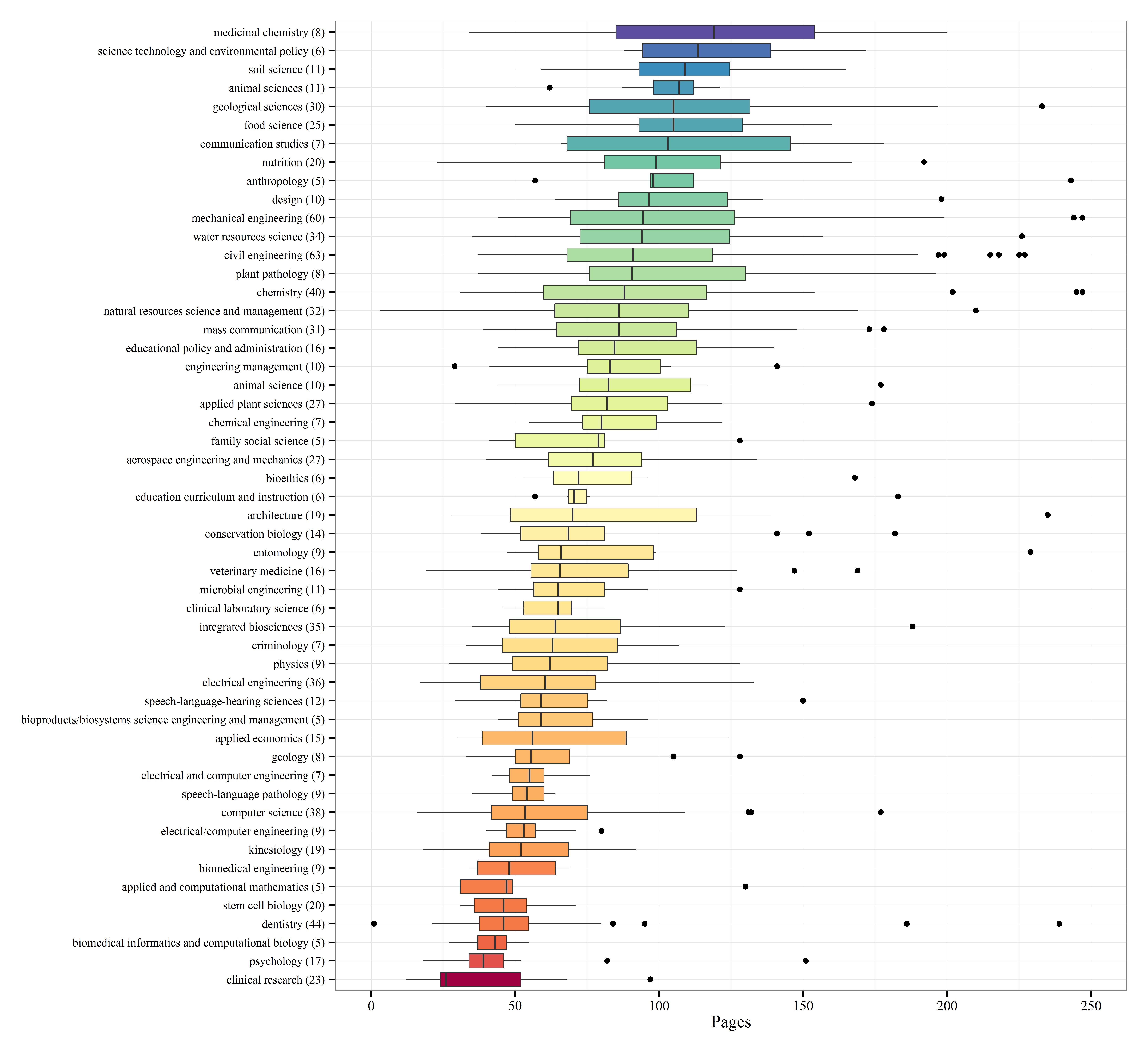
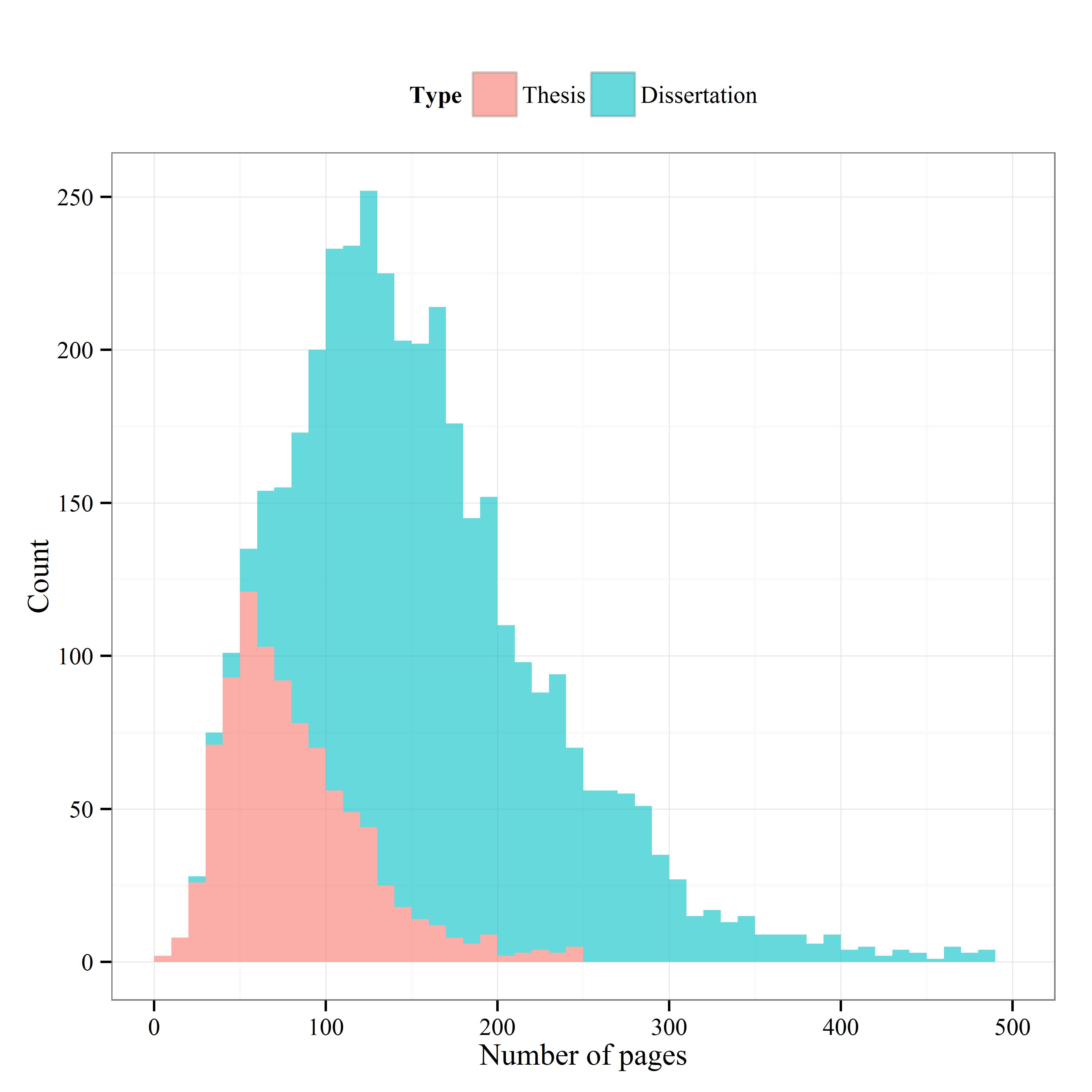
The data contained 2,536 records for students that completed their dissertations since 2007. The range was incredibly variable (minimum of 21 pages, maximum of 2002), but most dissertations were around 100 to 200 pages.

Interestingly, a lot of students graduated in August just prior to the fall semester. As expected, spikes in defense dates were also observed in December and May at the ends of the fall and spring semesters.

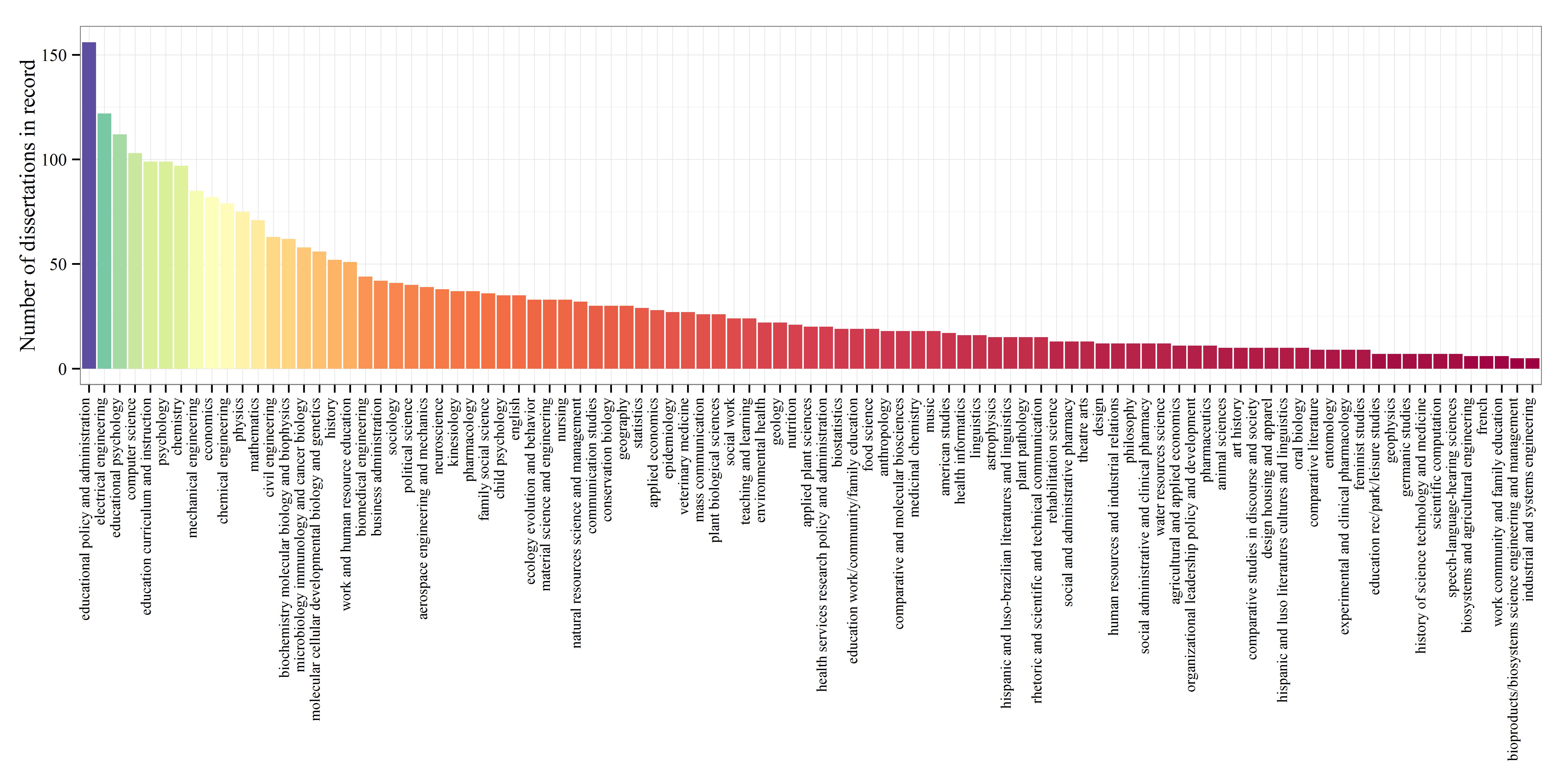
The top four majors with the most dissertations on record were (in descending order) educational policy and administration, electrical engineering, educational psychology, and psychology.

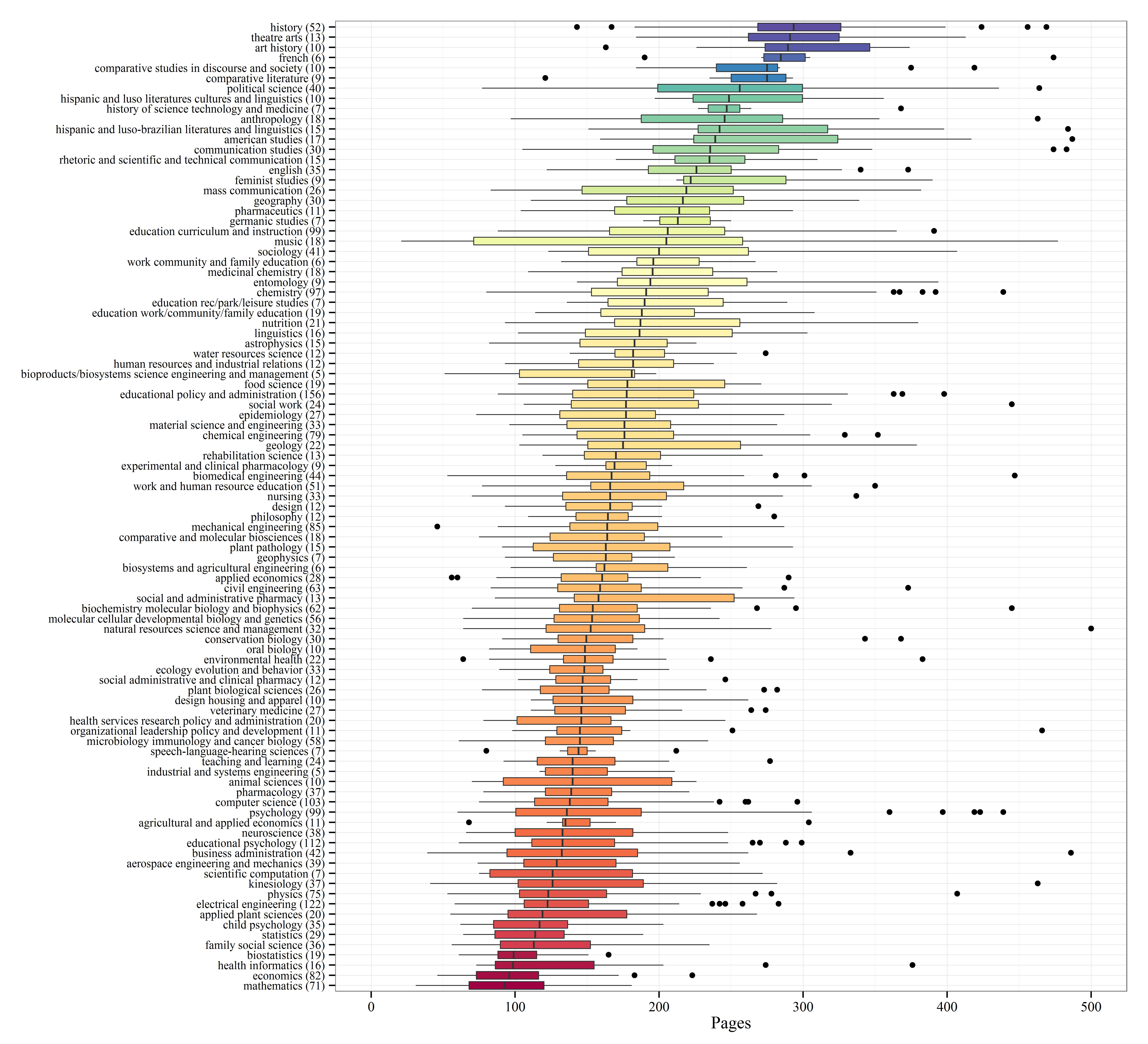
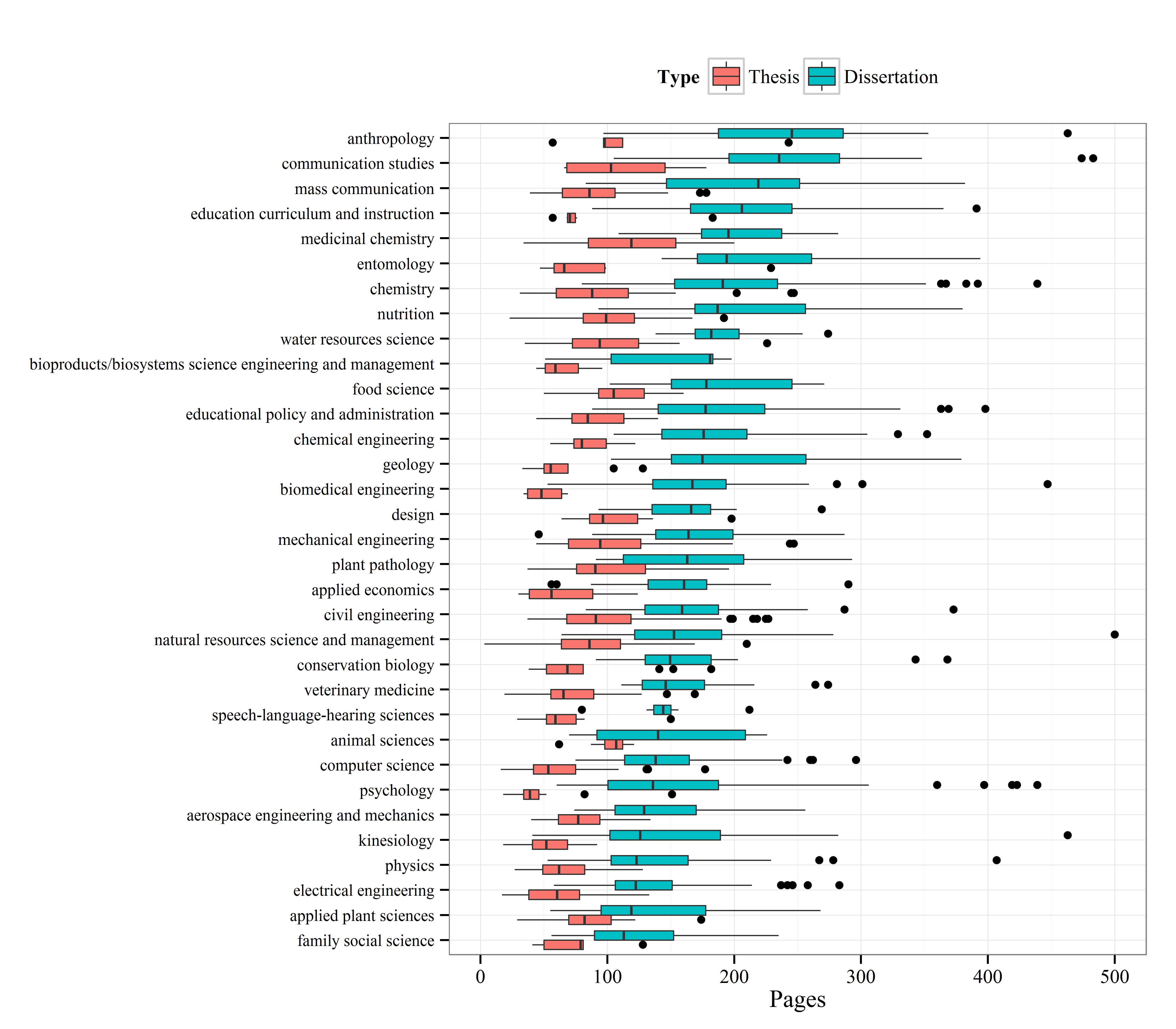
I’ve selected the top fifty majors with the highest number of dissertations and created boxplots to show relative distributions. Not many differences are observed among the majors, although some exceptions are apparent. Economics, mathematics, and biostatistics had the lowest median page lengths, whereas anthropology, history, and political science had the highest median page lengths. This distinction makes sense given the nature of the disciplines.

I’ve also completed a count of number of students per advisor. The maximum number of students that completed their dissertations for a single advisor since 2007 was eight. Anyhow, I’ve satiated my curiosity on this topic so it’s probably best that I actually work on my own dissertation rather than continue blogging. For those interested, the below code was used to create the plots.

######
#plot summary of data
require(ggplot2)

mean.val<-round(mean(check.pgs$pages))
med.val<-median(check.pgs$pages)
sd.val<-round(sd(check.pgs$pages))
rang.val<-range(check.pgs$pages)
txt.val<-paste('mean = ',mean.val,'\nmed = ',med.val,'\nsd = ',sd.val,
	'\nmax = ',rang.val[2],'\nmin = ', rang.val[1],sep='')

#histogram for all
hist.dat<-ggplot(check.pgs,aes(x=pages))
pdf('C:/Users/Marcus/Desktop/hist_all.pdf',width=7,height=5)
hist.dat + geom_histogram(aes(fill=..count..),binwidth=10) +
  scale_fill_gradient("Count", low = "blue", high = "green") +
	xlim(0, 500) + geom_text(aes(x=400,y=100,label=txt.val))
dev.off()

#barplot by month
month.bar<-ggplot(check.pgs,aes(x=month,fill=..count..))

pdf('C:/Users/Marcus/Desktop/month_bar.pdf',width=10,height=5.5)
month.bar + geom_bar() + scale_fill_gradient("Count", low = "blue", high = "green")
dev.off()

######
#histogram by most popular majors
#sort by number of dissertations by major
get.grps<-list(c(1:4),c(5:8))#,c(9:12),c(13:16))

for(val in 1:length(get.grps)){

	pop.maj<-names(sort(table(check.pgs$major),decreasing=T)[get.grps[[val]]])
	pop.maj<-check.pgs[check.pgs$major %in% pop.maj,]
	pop.med<-aggregate(pop.maj$pages,list(pop.maj$major),function(x) round(median(x)))
	pop.n<-aggregate(pop.maj$pages,list(pop.maj$major),length)

	hist.maj<-ggplot(pop.maj, aes(x=pages))
	hist.maj<-hist.maj + geom_histogram(aes(fill = ..count..), binwidth=10)
	hist.maj<-hist.maj + facet_wrap(~major,nrow=2,ncol=2) + xlim(0, 500) +
		scale_fill_gradient("Count", low = "blue", high = "green")

	y.txt<-mean(ggplot_build(hist.maj)$panel$ranges[[1]]$y.range)
	txt.dat<-data.frame(
		x=rep(450,4),
	  y=rep(y.txt,4),
		major=pop.med$Group.1,
		lab=paste('med =',pop.med$x,'\nn =',pop.n$x,sep=' ')
	  )

	hist.maj<-hist.maj + geom_text(data=txt.dat, aes(x=x,y=y,label=lab))

	out.name<-paste('C:/Users/Marcus/Desktop/group_hist',val,'.pdf',sep='')
	pdf(out.name,width=9,height=7)

	print(hist.maj)

	dev.off()

	}

######
#boxplots of data for fifty most popular majors

pop.maj<-names(sort(table(check.pgs$major),decreasing=T)[1:50])
pop.maj<-check.pgs[check.pgs$major %in% pop.maj,]

pdf('C:/Users/Marcus/Desktop/pop_box.pdf',width=11,height=9)
box.maj<-ggplot(pop.maj, aes(factor(major), pages, fill=pop.maj$major))
box.maj<-box.maj + geom_boxplot(lwd=0.5) + ylim(0,500) + coord_flip()
box.maj + theme(legend.position = "none", axis.title.y=element_blank())
dev.off()

Update: By popular request, I’ve redone the boxplot summary with major sorted by median page length.

Data fishing: R and XML part 3

I’ve recently posted two blogs about gathering data from web pages using functions in R. Both examples showed how we can create our own custom functions to gather data about Minnesota lakes from the Lakefinder website. The first post was an example showing the use of R to create our own custom functions to get specific lake information and the second was a more detailed example showing how we can get data on fish populations in each lake. Each of the examples used functions in the XML package to parse the raw XML/HTML from the web page for each lake. I promised to show some results using information that was gathered with the catch function described in the second post. The purpose of this blog is to present some of this information and to further illustrate the utility of data mining using public data and functions in R.

I’ll begin by describing the functionality of a revised catch function and the data that can be obtained. I’ve revised the original function to return more detailed information and decrease processing time, so this explanation is not a repeat of my previous blog. First, we import the function from Github with some help from the RCurl package.

#import function from Github
require(RCurl)

root.url<-'https://gist.github.com/fawda123'
raw.fun<-paste(
  root.url,
  '4978092/raw/336671b8c3d44f744c3c8c87dd18e6d871a3b370/catch_fun_v2.r',
  sep='/'
  )

script<-getURL(raw.fun, ssl.verifypeer = FALSE)
eval(parse(text = script))
rm('script','raw.fun')

#function name 'catch.fun.v2'

The revised function is much simpler than the previous and requires only three arguments.

formals(catch.fun.v2)
#dows

#$trace
#T

#$rich.out
#F

The ‘dows’ argument is a character vector of the 8-digit lake identifier numbers used by MNDNR, ‘trace’ is a logical specifying if progress is returned as the function runs, and ‘rich.out’ is a logical specifying if a character vector of all fish species is returned as a single element list. The ‘dows’ argument can process multiple lakes so long as you have the numbers. The default value for the last argument will return a list of two data frames with complete survey information for each lake.

I revised the original function after realizing that I’ve made the task of parsing XML for individual species much too difficult. The original function searches species names and gear type to find the appropriate catch data. A simpler approach is to find the entire survey table by parsing with <table></table> tags. The original function parsed the XML using <tr></tr> tags for table rows and then identified the appropriate species and gear type within the rows. The latter approach required multiple selection criteria and was incredibly inefficient. The new function returns entire tables, which can be further modified within R as needed. Here’s an example for Loon lake in Aitkin county.

catch.fun.v2('01002400')

#01002400; 1 of 1 
#Time difference of 1.844106 secs
#$`01002400`
#$`01002400`$abundance
#Species        Net Caught Ave_wt
#1  White Sucker  Trap net     0.1   ND  
#2 Rainbow Trout  Trap net   trace   ND  
#3   Brook Trout  Trap net     4.6   ND  

#$`01002400`$length
#Species   0-5   6-8  9-11 12-14 15-19
#1   Brook Trout     0    28    36    22     3
#2 Rainbow Trout     0     0     0     1     0
#20-24 25-29   30+  Total
#1     0     0     0     89
#2     0     0     0      1

This is the same information that is on the lakefinder website. A two-element list is returned for each lake, each containing a data frame. The first element is a data frame of species catch (fish per net) and average weight (lbs per fish) using trap nets and gill nets (this example only contained trap nets). The second element is a length distribution table showing the number of fish caught within binned length categories (inches). A character string specifying ‘No survey’ will be returned if the lake isn’t found on the website or if no fish surveys are available. A character string indicating ‘No length table’ will be returned in the second list element if only the abundance table is available.

A list of the species present is returned if ‘rich.out’ is true.

catch.fun.v2('01002400',rich.out=T)

#01002400; 1 of 1 
#Time difference of 0.419024 secs
#$`01002400`
#[1] "Brook Trout"   "Rainbow Trout"
#[3] "White Sucker" 

Clearly the utility of this function is the ability to gather lake data for multiple lakes without visiting each individual page on Lakefinder. I’ve used the function to get lake data for every lake on the website. The dow numbers were obtained from a publicly available shapefile of lakes in Minnesota. This included 17,085 lakes, which were evaluated by the function in less than an hour. Of these lakes, 3,934 had fish survey information. One drawback of the function is that I haven’t included the date of the survey in the output (updated, see link at bottom of blog). The data that are returned span several years, and in some cases, the most recent lake survey could have been over 40 years ago.

Below is a presentation of some of the more interesting information obtained from the data. First, I’ve included two tables that show the top five lakes for abundance and average weight for two popular game fish. The tables are separated by gear type since each targets different habitats. Keep in mind that this information may not represent the most current population data.

Top five lakes in Minnesota for catch (fish per net) and average weight (lbs per fish) of walleye separated by net type.
Net type DOW Name County Caught Ave_wt
Gill 21014500 Chippewa Douglas 9.92
9005700 Eagle Carlton 9.89
69073100 Auto  St. Louis 9.75
31089600 Round  Itasca 9.67
47011900 Minnie Belle Meeker 9.67
11011400 Mitten Cass 9.38
31079300 Big Too Much Itasca 8.86
9004300 Moose Carlton 8.05
11019900 Hay Cass 7.82
11017700 Three Island Cass 7.61
Trap 87001900 Tyson Yellow Medicine 9.67
69019000 Big St. Louis 8.5
16025300 Deer Yard Cook 7.55
16064500 Toohey Cook 7.33
51004600 Shetek Murray 7.27
69017400 East Twin St. Louis 9.04
21016200 Freeborn Douglas 8.65
31054700 Smith Itasca 8.39
69054400 Dinham St. Louis 8.38
82002300 Lily Washington 8.11
Top five lakes in Minnesota for catch (fish per net) and average weight (lbs per fish) of northern pike separated by net type.
Net type DOW Name County Caught Ave_wt
Gill 4019600 Campbell Beltrami 9.89
11017400 Girl Cass 9.89
56091500 Prairie Otter Tail 9.83
69051300 Little Grand St. Louis 9.83
34015400 Nest Kandiyohi 9.8
38022900 Little Knife Lake 9.27
7007900 Benz Todd 9.16
29018400 Blue Hubbard 8.56
18043700 Portsmouth Mine Crow Wing 8.39
69011600 Mitchell St. Louis 8.3
Trap 61002900 Westport  Pope 9.56
16024800 Ward Cook 5.17
11028400 Horseshoe Cass 4.56
16025000 Mark Cook 4.33
62005500 Como Ramsey 4
9001600 Hay Hubbard 9.96
27018100 Dutch Hennepin 8.86
27001600 Harriet Hennepin 8.61
34003300 Ella Kandiyohi 8.6
34007900 Green Kandiyohi 8.6

The above tables illustrate the value of the information that can be obtained using data mining techniques in R, even though most anglers are already aware of the best fishing lakes in Minnesota. A more comprehensive assessment of the data on Lakefinder is shown below. The fist two figures show species richness and total biomass (lbs per net) for the approximate 4000 lakes with fish surveys. Total biomass for each lake was the summation of the product of average weight per fish and fish per net for all species using gill net data. Total biomass can be considered a measure of lake productivity, although in many cases, this value is likely determined by a single species with high abundance (e.g., carp or bullhead).

Summary of species richness (count) and total biomass (lbs per net) for lakes in Minnesota.

The next two figures show average species richness and total biomass for each county. Individual values for each county are indicated.

Summary of species richness (count) and total biomass (lbs per net) for lakes in Minnesota.

We see some pretty interesting patterns when we look at the statewide data. In general, species richness and biomass decreases along a southwest to northeast direction. These patterns vary in relation to the trophic state or productivity of each lake. We can also develop some interesting ecological hypotheses for the observed relationships. The more important implication for R users is that we’ve gathered and summarized piles of data from publicly available sources, data which can generate insight into causation. Interestingly, the maps were generated in R using the proprietary shapefile format created for ArcMap. The more I explore the packages in R that work with spatial data (e.g., sp, raster, maptools), the less I have worked with ArcMap. I’ve gone to great lengths to convince myself that the application of data mining tools available in R provide a superior alternative to commercial software. I hope that these simple examples have convinced you as well.

You can access version 2 of the catch function with the above code via my Github account. I’ve provided the following code to illustrate how the maps were produced. The data for creating the maps are not provided because this information can be obtained using the examples in this blog.

##
#first figure, summary of species richness and biomass for ~4000 lakes

require(raster)
require(sp)
require(maptools)
require(RColorBrewer) #for color ramps
require(scales) #for scaling points

par(mfrow=c(1,2),mar=numeric(4),family='serif')

#species richness
plot(counties,col='lightgrey') #get county shapefile from DNR data deli, link in blog

col.fun<-colorRampPalette(brewer.pal(11,'RdYlBu'))
col.pts<-rev(col.fun(nrow(lake.pts)))[rank(lake.pts$spp_rich)] #lake.pts can be created using 'catch.fun.v2'
rsc.pts<-rescale(lake.pts$spp_rich,c(0.5,5))
points(lake.pts$UTM_X,lake.pts$UTM_Y,cex=rsc.pts,col=col.pts,pch=19)
title(sub='Species richness per lake',line=-2,cex.sub=1.5)

leg.text<-as.numeric(summary(lake.pts$spp_rich))[-4]
leg.cex<-seq(0.5,5,length=5)
leg.col<-rev(col.fun(5))
legend(650000,5250000,legend=leg.text,pt.cex=leg.cex,col=leg.col,
       title='',pch=19,bty='n', cex=1.4,y.intersp=1.4,inset=0.11)

#scale bar
axis(side=3,
     at=c(420000,520000,620000),
     line=-4,labels=c('0 km','100 km','200 km'),
     cex.axis=1
  )

#total biomass
plot(counties,col='lightgrey')

col.fun<-colorRampPalette(brewer.pal(11,'RdYlBu'))
col.pts<-rev(col.fun(nrow(lake.pts)))[rank(lake.pts$ave.bio)]
rsc.pts<-rescale(lake.pts$ave.bio,c(0.5,5))
points(lake.pts$UTM_X,lake.pts$UTM_Y,cex=rsc.pts,col=col.pts,pch=19)
title(sub='Total biomass per lake (lbs/net)',line=-2,cex.sub=1.5)

leg.text<-as.numeric(summary(lake.pts$ave.bio))[-4]
leg.cex<-seq(0.5,5,length=5)
leg.col<-rev(col.fun(5))
legend(650000,5250000,legend=leg.text,pt.cex=leg.cex,col=leg.col,
       title='',pch=19,bty='n', cex=1.4,y.intersp=1.4,inset=0.11)

##
#second figure, county summaries

lake.pts.sp<-lake.pts #data from combination of lake polygon shapefile and catch data from catch.fun.v2
coordinates(lake.pts.sp)<-cbind(lake.pts.sp$UTM_X,lake.pts.sp$UTM_Y)

test<-over(counties,lake.pts.sp[,c(7,10)],fn=mean) #critical function for summarizing county data

co.rich<-test[,'spp_rich']
co.bio<-test[,'ave.bio']

my.cols<-function(val.in){
  pal<-colorRampPalette(brewer.pal(11,'RdYlBu')) #create color vector
  out<-numeric(length(val.in))
  out[!is.na(val.in)]<-rev(pal(sum(!is.na(val.in))))[rank(val.in[!is.na(val.in)])]  
  out[out=='0']<-'lightgrey'
  out
}

#make plots
par(mfrow=c(1,2),mar=numeric(4),family='serif')
plot(counties,col=my.cols(co.rich))
text.coor<-coordinates(counties)[!is.na(co.rich),]
text(text.coor[,1],text.coor[,2],format(co.rich[!is.na(co.rich)],nsmall=1,
     digits=1),cex=0.8)
axis(side=3,
     at=c(420000,520000,620000),
     line=-4,labels=c('0 km','100 km','200 km'),
     cex.axis=1
)
title(sub='Average species richness by county',line=-2,cex.sub=1.5)

plot(counties,col=my.cols(co.bio))
text.coor<-coordinates(counties)[!is.na(co.bio),]
text(text.coor[,1],text.coor[,2],format(co.bio[!is.na(co.bio)],nsmall=1,
     digits=1),cex=0.8)
title(sub='Average biomass by county',line=-2,cex.sub=1.5)

Update: I’ve updated the catch function to return survey dates.

Data fishing: R and XML part 2

I’m constantly amazed at what can be done using free software, such as R, and more importantly, what can be done with data that are available on the internet. In an earlier post, I confessed to my sedentary lifestyle immersed in code, so my opinion regarding the utility of open-source software is perhaps biased. None the less, I’m convinced that more people would start using and continue to use R once they’ve realized the limitless applications.

My first post highlighted what can be done using the XML package, or more generally, what can be done ‘stealing’ data from the internet using free software and publicly available data. I return to this concept in this blog to show you, and hopefully convince you, that learning how to code your own functions for data mining is a worthwhile endeavor. My last example showed how we can get depth data for lakes from the Lakefinder website maintained by the Minnesota Department of Natural Resources. I’ll admit the example was boring and trivial, but my intention was to introduce the concept as the basis for further blogs. The internet contains an over-abundance of information and R provides several useful tools to gather and analyze this information.

After seeing this post about data mining with Twitter (check the video!), I was motivated to create a more interesting example than my previous posting using LakeFinder. Minnesota, the land of 11,842 lakes, has some of the best fishing in the country. The ostensible purpose of Lakefinder is to provide anglers access to lake data gathered by MNDNR. Most people don’t care about lake depth, so I developed a more flexible function that accesses data from fish surveys. The fisheries division at MNDNR collects piles and piles of fish data and Lakefinder should have the most current survey information for managed lakes (although I don’t know how often the data are updated). Each year, local offices conduct trap net surveys in nearshore areas and gill net surveys to sample fish in open water. An example of the data is shown for Christmas Lake under ‘Fish Sampled for the 2007 Survey Year’. Species are listed in each row and species catch is listed in the columns. Fish per net can be considered a measure of abundance and is often correlated with angler catch. Lakes with higher fish per net, in either trap or gill nets, likely have better fishing.

The purpose of this blog is to describe a custom R function for gathering information about fish catch off LakeFinder. Those outside of Minnesota will have little use for the data gathered by this function. However, I think the most important implication is that anyone with a computer has the potential to develop customized functions to gather a potentially limitless amount of information from the internet. I hope the results I’ve obtained using this function will convince you of this fact. I’ll save the juicy tidbits for my next blog (where are the best lakes?).

What started as a straightforward idea quickly turned into a rather nasty problem handling exceptions when the website contained information that didn’t match the search criteria used in the function. The trick to writing a useful function is to incorporate enough flexibility so that it can accommodate all cases or forms of the data. For example, a function that can only process data frames will fail if it tries to process a list. This concept is central to programming and helps us understand why the fish catch function seems so complex. I had to create a function that could handle every instance in the fish catch table for each lake where the species data existed in a form that made it unambiguous to identify (i.e., it was obvious that the species was or was not in the survey for a given gear type).

Here are some examples illustrating how the function can identify the correct species and net type for each lake:

Fish name Net type Catch
Bluegill Gill 0.6
Northern Pike Trap 12.2
Bluegill Trap 32.1
Walleye Gill 12.6

This example is easy enough if we are looking for bluegill in trap nets. All we have to is pull out the rows with Bluegill in the first column, then identify the row with the correct net type, and append the value in the third column to our output. The next example illustrates a case that isn’t so clear.

Fish name Net type Catch
Bluegill Gill 0.6
Trap 32.1
Northern Pike Trap 12.2
Walleye Gill 12.6

Say we’ve written the function to identify fish and net data using only criteria that can handle data in the first table. We run into problems if we apply the same criteria to identify the catch of bluegill in trap nets for the second table (a common form for the Lakefinder survey data). We can’t identify all bluegill rows using species name in the first column since it isn’t labelled for trap nets. Nor can we identify bluegill based on our designated net type (Northern Pike were also caught in trap nets). One workaround is to pull out the single row with Bluegill and the following row. Then we can check which row of the two contains trap nets in the second column This assumes an empty row name for species is bluegill, which is a valid assumption considering data in the previous row are for bluegill. What if the species column for the row below bluegill isn’t blank and contains another species? We can’t use our ‘bluegill + next row’ rule, so we have to incorporate further selection techniques to reach an unambiguous solution. Hopefully you can see how complexity quickly emerges from what initially seemed like a simple task.

The final code for the function incorporated eight different selection methods based on how the data were presented on Lakefinder. The code is pretty nasty-looking, so here’s a flowchart that shows what the function does.

my image

Here’s what it looks like to use the function in R:

#create string of lake ids to search
dows.in<-c('27013700','82004600','82010400')

#create string of fish names to search
fish.names<-c('Bluegill','Largemouth Bass','Northern Pike')

#use the function
catch.fun(dows=dows.in, fish.str=fish.names, net.type='Trap', trace=T, clean=F)

There are five arguments for catch.fun. The first two are required and the last three have default values. ‘dows’ is a string of lake DOW numbers that identify the lakes you want to search (these numbers are available on the DNR Data Deli). ‘fish.str’ is a string of common fish names that will be searched. The ‘net.type’ is a string that specifies whether you want to search trap net (default) or gill net data (as ‘Trap’ or ‘Gill’). ‘trace’ is a logical argument that indicates if text showing progress will be returned as the function runs. Finally, ‘clean’ is a logical argument that indicates if the function will return output with only lake and fish data. I’ll explain in a bit why I included this last argument.

Now some details (skip if you’re bored)… the flowchart indicates that the fish names in ‘fish.str’ are searched for each lake in ‘dows’ using a nested loop with lake dow at the top level and fish name at the bottom level (denoted by the dotted line box). The tricky part comes when we have to deal with the different forms of the data I mentioned earlier. The flowchart has several hexagonal decision nodes that determine how the data are interpreted in the function. Each time the function reaches an unambiguous result, the yes/no decisions include an exception code (‘e1’ through ‘e8’) that specifies the form of the data that was found. Starting with the first exception (‘e1’), we can see what is meant by terminal. An ‘e1’ is returned while searching a lake DOW if the lake doesn’t exist on LakeFinder or if a lake exists but the survey isn’t available. If the lake and survey both exist, the function jumps into the loop through each species. The first check within the fish loop determines if the fish being searched is present in the survey. If not, ‘e2’ (second exception) is entered for the species and the loop continues to the next. Zero values are returned if a fish isn’t in a survey, otherwise NA is returned for no survey or no lake data. The function continues through several more decision nodes until a final result for each species in each lake is obtained.

Finally, I included a safety measure that allows the function to continue running if some unforeseen issue is encountered (‘massive failure’). This exception (‘e8’) will be returned if an error occurs at any point during the fish search. This only occurred once because someone had entered two species names for the same fish and same net type in the same lake (unresolved, unforeseen ambiguity). Its a good idea to include safety nets in your functions because its very difficult to be 100% certain the function captures all exceptions in the data. Rather than having the function crash, the error is noted and the function continues.

Alright, enough of that. Let’s see what the function returns. Using the above code, we get the catch for the three lakes based on the net type and species we wanted to find:

catch.fun(dows=dows.in, fish.str=fish.names, net.type='Trap', trace=T, clean=F)

27013700; 1 of 3 
82004600; 2 of 3 
82010400; 3 of 3 
Time difference of 1.368078 secs
$Bluegill
      dows     fish fish.val result
1 27013700 Bluegill    51.22     e6
2 82004600 Bluegill     9.22     e6
3 82010400 Bluegill    43.56     e6

$`Largemouth Bass`
      dows            fish fish.val result
4 27013700 Largemouth Bass     1.44     e6
5 82004600 Largemouth Bass        0     e7
6 82010400 Largemouth Bass     0.44     e6

$`Northern Pike`
      dows          fish fish.val result
7 27013700 Northern Pike     0.44     e6
8 82004600 Northern Pike     1.33     e6
9 82010400 Northern Pike     2.11     e6

The function returns a list for each species with data frames in each element of the list. The columns of each data frame include the lake name, species (which is redundant), the catch for the specified net type (number of fish per net), and the final decision in the function that lead to the result. I included the ‘result’ column in the data so I could see if the function was actually doing what it was supposed to do. You get cleaner results if you set ‘clean’ as true, obviously. The output will have the result column and the redundant fish column in the data frames removed. Lakes not in Lakefinder or lakes without fish surveys will also be removed.

I’ve covered the nitty-gritty of what the function does and how it can be used. The data that can be gathered are of course more interesting than the function and I save a presentation of this material for my next blog. For now, here’s a teaser showing presence/absence of common carp using data obtained with the function. Common carp (not Asian) are ubiquitous in Minnesota and anglers may be interested in carp locations based on the impacts invasive fish have on native species. We can use the function to locate all the lakes surveyed by Minnesota DNR that contain common carp. Thanks to our data fishing we now know to avoid common carp by fishing up north. Stay tuned for the next installment!

Get the function here (requires XML package):

catch.fun<-function(dows,fish.str,net.type='Trap',trace=T,clean=F){
require(XML)
strt<-Sys.time()
#create object for output
fish.out<-data.frame(expand.grid(dows,fish.str),NA,NA)
names(fish.out)<-c('dows','fish','fish.val','result')
for(dow in dows){
if(trace){
cat(paste(dow,'; ',which(dow==dows),' of ',length(dows),sep=''),'\n')
flush.console()
}
#get raw html
html<-htmlTreeParse(
paste(
'http://www.dnr.state.mn.us/lakefind/showreport.html?downum=&#39;,
dow,
'&qitem=DOWLKNUM_1',
sep=''
),
useInternalNodes=TRUE
)
#exception 1, no site for dow or no fish survey
check.site<-unlist(xpathApply(html, "//h3", xmlValue))
if(length(grep('Fish Sampled*',check.site))==0){
fish.out[dows==dow,4]<-'e1'
next
}
#survey exists, get survey data
#exception for surveys with only one table
#replace trace with zero
fish.tab<-unlist(xpathApply(html, "//tr", xmlValue))
fish.row<-grep('Species*',fish.tab)[1:2]
if(is.na(fish.row[2])) fish.row[2]<-grep('\nFor more information',fish.tab)
fish.tab<-fish.tab[fish.row[1]:fish.row[2]]
fish.tab<-gsub('trace','0',fish.tab)
if(class(try(
for(fish in fish.str){
#does fish exist in the table?
fish.row<-grep(paste('*',fish,'*',sep=''),fish.tab)
#row in output data.frame to fill, logical vector
out.row<-fish.out$dows==dow & fish.out$fish==fish
#exception 2, fish survey but spp not found
if(length(fish.row)==0){
fish.out[out.row,3:4]<-c(0,'e2')
next
}
#exception 3, fish found, two rows with spp label each row
if(length(fish.row)==2){
fish.val<-strsplit(
grep(net.type,fish.tab[fish.row],value=T),'\n'
)[[1]][3]
fish.out[out.row,3:4]<-c(fish.val,'e3')
next
}
check.rows<-fish.tab[c(fish.row,fish.row+1)]
check.net<-grepl(net.type,check.rows)
#exception 4, fish found, one row with fish label, net type not found
if(sum(check.net)==0){
fish.out[out.row,3:4]<-c(0,'e4')
next
}
#exception 5, fish found, one row with fish label,
#net type found in both rows
if(sum(check.net)==2){
fish.val<-strsplit(check.rows[1],'\n')[[1]][3]
fish.out[out.row,3:4]<-c(fish.val,'e5')
next
}
final.row<-strsplit(check.rows[check.net],'\n')[[1]]
#exception 6, fish found, one row with fish label,
#net type found in one row, row with net is for correct species
#(less than three characters or contains species name)
if(nchar(final.row[1])<3 | final.row[1]==fish){
fish.val<-final.row[3]
fish.out[out.row,3:4]<-c(fish.val,'e6')
next
}
#exception 7, fish found, one row with fish label,
#net type found in one row
fish.out[out.row,3:4]<-c(0,'e7')
}
))=='try-error'){
#exception 8, unknown
fish.out[fish.out$dows==dow,4]<-'e8'
}
}
fish.out<-split(fish.out,fish.out$fish)
print(Sys.time()-strt)
if(clean) return(lapply(fish.out,function(x) x[!is.na(x[,3]),-c(2,4)]))
fish.out
}
view raw catch_fun.r hosted with ❤ by GitHub