
Collinearity, or excessive correlation among explanatory variables, can complicate or prevent the identification of an optimal set of explanatory variables for a statistical model. For example, forward or backward selection of variables could produce inconsistent results, variance partitioning analyses may be unable to identify unique sources of variation, or parameter estimates may include substantial amounts of uncertainty. The temptation to build an ecological model using all available information (i.e., all variables) is hard to resist. Lots of time and money are exhausted gathering data and supporting information. We also hope to identify every significant variable to more accurately characterize relationships with biological relevance. Analytical limitations related to collinearity require us to think carefully about the variables we choose to model, rather than adopting a naive approach where we blindly use all information to understand complexity. The purpose of this blog is to illustrate use of some techniques to reduce collinearity among explanatory variables using a simulated dataset with a known correlation structure.
A simple approach to identify collinearity among explanatory variables is the use of variance inflation factors (VIF). VIF calculations are straightforward and easily comprehensible; the higher the value, the higher the collinearity. A VIF for a single explanatory variable is obtained using the r-squared value of the regression of that variable against all other explanatory variables:

where the 


Several packages in R provide functions to calculate VIF: vif in package HH, vif in package car, VIF in package fmsb, vif in package faraway, and vif in package VIF. The number of packages that provide VIF functions is surprising given that they all seem to accomplish the same thing. One exception is the function in the VIF package, which can be used to create linear models using VIF-regression. The nuts and bolts of this function are a little unclear since the documentation for the package is sparse. However, what this function does accomplish is something that the others do not: stepwise selection of variables using VIF. Removing individual variables with high VIF values is insufficient in the initial comparison using the full set of explanatory variables. The VIF values will change after each variable is removed. Accordingly, a more thorough implementation of the VIF function is to use a stepwise approach until all VIF values are below a desired threshold. For example, using the full set of explanatory variables, calculate a VIF for each variable, remove the variable with the single highest value, recalculate all VIF values with the new set of variables, remove the variable with the next highest value, and so on, until all values are below the threshold.
In this blog we’ll use a custom function for stepwise variable selection. I’ve created this function because I think it provides a useful example for exploring stepwise VIF analysis. The function is a wrapper for the vif function in fmsb. We’ll start by simulating a dataset with a known correlation structure.
require(MASS)
require(clusterGeneration)

set.seed(2)
num.vars<-15
num.obs<-200
cov.mat<-genPositiveDefMat(num.vars,covMethod="unifcorrmat")$Sigma
rand.vars<-mvrnorm(num.obs,rep(0,num.vars),Sigma=cov.mat)
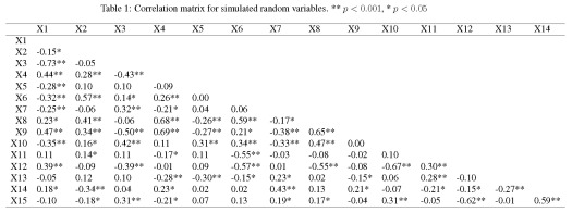
We’ve created fifteen ‘explanatory’ variables with 200 observations each. The mvrnorm function (MASS package) was used to create the data using a covariance matrix from the genPositiveDefMat function (clusterGeneration package). These functions provide a really simple approach to creating data matrices with arbitrary correlation structures. The covariance matrix was chosen from a uniform distribution such that some variables are correlated while some are not. A more thorough explanation about creating correlated data matrices can be found here. The correlation matrix for the random variables should look very similar to the correlation matrix from the actual values (as sample size increases, the correlation matrix approaches cov.mat).
Now we create our response variable as a linear combination of the explanatory variables. First, we create a vector for the parameters describing the relationship of the response variable with the explanatory variables. Then, we use some matrix algebra and a randomly distributed error term to create the response variable. This is the standard form for a linear regression model.
parms<-runif(num.vars,-10,10)
y<-rand.vars %*% matrix(parms) + rnorm(num.obs,sd=20)
We would expect a regression model to indicate each of the fifteen explanatory variables are significantly related to the response variable, since we know the true relationship of y with each of the variables. However, our explanatory variables are correlated. What happens when we create the model?
lm.dat<-data.frame(y,rand.vars)
form.in<-paste('y ~',paste(names(lm.dat)[-1],collapse='+'))
mod1<-lm(form.in,data=lm.dat)
summary(mod1)
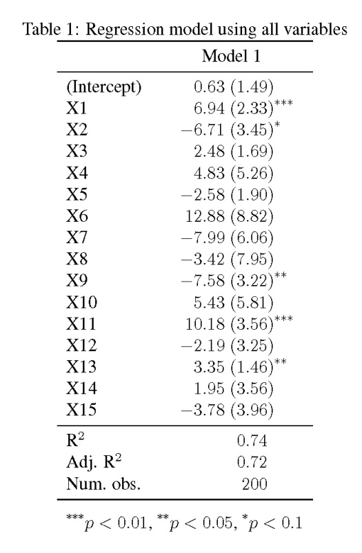
The model shows that only four of the fifteen explanatory variables are significantly related to the response variable (at 
We can try an alternative approach to building the model that accounts for collinearity among the explanatory variables. We can implement the custom VIF function as follows.
vif_func(in_frame=rand.vars,thresh=5,trace=T)

 var vif
 X1  27.7352782054202
 X2  36.8947196546879
 X3  12.5694198086941
 X4  50.7385544899845
 X5  8.35069942629285
 X6  114.685122241139
 X7  67.3415420139211
 X8  153.597012767649
 X9  48.226662808638
 X10 50.7371404106266
 X11 33.9720046917178
 X12 43.2541022358368
 X13 12.0823286959991
 X14 74.6186892947576
 X15 29.8722459010406

removed:  X8 153.597

 var vif
 X1  6.67306561938667
 X2  7.98347501302268
 X3  4.56187657632574
 X4  8.03048468634153
 X5  7.70736760805487
 X6  19.6743072270573
 X7  52.9521670096974
 X9  17.8683960730445
 X10 46.2484642889962
 X11 18.2479446141727
 X12 42.133697798185
 X13 10.8973377491163
 X14 37.9296952803818
 X15 21.5847028917955

removed:  X7 52.95217

 var vif
 X1  6.54376168051204
 X2  7.68236114754164
 X3  4.04873004990332
 X4  5.08958904348524
 X5  2.65685239947949
 X6  9.12685384862522
 X9  2.89940351012031
 X10 4.24712217472346
 X11 4.45202381077724
 X12 12.8835110845825
 X13 1.92759852488083
 X14 6.02382346000219
 X15 8.33332235677386

removed:  X12 12.88351

 var vif
 X1  4.21690743815539
 X2  6.88058249786417
 X3  3.88265091747854
 X4  4.48146995293666
 X5  2.20144300270463
 X6  7.76775127218149
 X9  2.71324446993905
 X10 2.90517847805482
 X11 4.43541888871566
 X13 1.78221291029774
 X14 5.02289299193397
 X15 3.02196822776011

removed:  X6 7.767751

 [1] "X1"  "X2"  "X3"  "X4"  "X5"  "X9"  "X10" "X11" "X13" "X14" "X15"
The function uses three arguments. The first is a matrix or data frame of the explanatory variables, the second is the threshold value to use for retaining variables, and the third is a logical argument indicating if text output is returned as the stepwise selection progresses. The output indicates the VIF values for each variable after each stepwise comparison. The function calculates the VIF values for all explanatory variables, removes the variable with the highest value, and repeats until all VIF values are below the threshold. The final output is a list of variable names with VIF values that fall below the threshold. Now we can create a linear model using explanatory variables with less collinearity.
keep.dat<-vif_func(in_frame=rand.vars,thresh=5,trace=F)
form.in<-paste('y ~',paste(keep.dat,collapse='+'))
mod2<-lm(form.in,data=lm.dat)
summary(mod2)
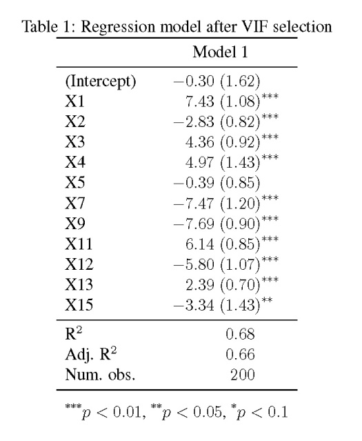
The updated regression model is much improved over the original. We see an increase in the number of variables that are significantly related to the response variable. This increase is directly related to the standard error estimates for the parameters, which look at least 50% smaller than those in the first model. The take home message is that true relationships among variables will be masked if explanatory variables are collinear. This creates problems in model creation which lead to complications in model inference. Taking the extra time to evaluate collinearity is a critical first step to creating more robust ecological models.
Function and example code:
| vif_func<-function(in_frame,thresh=10,trace=T,wts=NULL,...){ | |
| library(fmsb) | |
| if(any(!'data.frame' %in% class(in_frame))) in_frame<-data.frame(in_frame) | |
| if(is.null(wts)) | |
| wts <- rep(1, ncol(in_frame)) | |
| if(!is.null(wts)) | |
| if(length(wts)!=ncol(in_frame)) stop('length of weights must equal number of variables') | |
| if(any(wts < 0)) | |
| stop('weights must be positive') | |
| names(wts) <- names(in_frame) | |
| #get initial vif value for all comparisons of variables | |
| vif_init<-NULL | |
| var_names <- names(in_frame) | |
| for(val in var_names){ | |
| wt <- wts[val] | |
| regressors <- var_names[-which(var_names == val)] | |
| form <- paste(regressors, collapse = '+') | |
| form_in <- formula(paste(val, '~', form)) | |
| vif_init<-rbind(vif_init, c(val, VIF(lm(form_in, data = in_frame, ...)) / wt)) | |
| } | |
| vif_max<-max(as.numeric(vif_init[,2]), na.rm = TRUE) | |
| if(vif_max < thresh){ | |
| if(trace==T){ #print output of each iteration | |
| prmatrix(vif_init,collab=c('var','vif'),rowlab=rep('',nrow(vif_init)),quote=F) | |
| cat('\n') | |
| cat(paste('All variables have VIF < ', thresh,', max VIF ',round(vif_max,2), sep=''),'\n\n') | |
| } | |
| return(var_names) | |
| } | |
| else{ | |
| in_dat<-in_frame | |
| #backwards selection of explanatory variables, stops when all VIF values are below 'thresh' | |
| while(vif_max >= thresh){ | |
| vif_vals<-NULL | |
| var_names <- names(in_dat) | |
| for(val in var_names){ | |
| wt <- wts[val] | |
| regressors <- var_names[-which(var_names == val)] | |
| form <- paste(regressors, collapse = '+') | |
| form_in <- formula(paste(val, '~', form)) | |
| vif_add<- VIF(lm(form_in, data = in_dat, ...)) / wt | |
| vif_vals<-rbind(vif_vals,c(val,vif_add)) | |
| } | |
| max_row<-which(vif_vals[,2] == max(as.numeric(vif_vals[,2]), na.rm = TRUE))[1] | |
| vif_max<-as.numeric(vif_vals[max_row,2]) | |
| if(vif_max<thresh) break | |
| if(trace==T){ #print output of each iteration | |
| prmatrix(vif_vals,collab=c('var','vif'),rowlab=rep('',nrow(vif_vals)),quote=F) | |
| cat('\n') | |
| cat('removed: ',vif_vals[max_row,1],vif_max,'\n\n') | |
| flush.console() | |
| } | |
| in_dat<-in_dat[,!names(in_dat) %in% vif_vals[max_row,1], drop = F] | |
| if(ncol(in_dat)==1) break | |
| } | |
| return(names(in_dat)) | |
| } | |
| } |
