Visualizing neural networks from the nnet package

Note: Please see the update to this post!

Neural networks have received a lot of attention for their abilities to ‘learn’ relationships among variables. They represent an innovative technique for model fitting that doesn’t rely on conventional assumptions necessary for standard models and they can also quite effectively handle multivariate response data. A neural network model is very similar to a non-linear regression model, with the exception that the former can handle an incredibly large amount of model parameters. For this reason, neural network models are said to have the ability to approximate any continuous function.

I’ve been dabbling with neural network models for my ‘research’ over the last few months. I’ll admit that I was drawn to the approach given the incredible amount of hype and statistical voodoo that is attributed to these models. After working with neural networks, I’ve found that they are often no better, and in some cases much worse, than standard statistical techniques for predicting relationships among variables. Regardless, the foundational theory of neural networks is pretty interesting, especially when you consider how computer science and informatics has improved our ability to create useful models.

R has a few packages for creating neural network models (neuralnet, nnet, RSNNS). I have worked extensively with the nnet package created by Brian Ripley. The functions in this package allow you to develop and validate the most common type of neural network model, i.e, the feed-forward multi-layer perceptron. The functions have enough flexibility to allow the user to develop the best or most optimal models by varying parameters during the training process. One major disadvantage is an inability to visualize the models. In fact, neural networks are commonly criticized as ‘black-boxes’ that offer little insight into causative relationships among variables. Recent research, primarily in the ecological literature, has addressed this criticism and several approaches have since been developed to ‘illuminate the black-box’.¹

As far as I know, none of the recent techniques for evaluating neural network models are available in R. Özesmi and Özemi (1999)² describe a neural interpretation diagram (NID) to visualize parameters in a trained neural network model. These diagrams allow the modeler to qualitatively examine the importance of explanatory variables given their relative influence on response variables, using model weights as inference into causation. More specifically, the diagrams illustrate connections between layers with width and color in proportion to magnitude and direction of each weight. More influential variables would have lots of thick connections between the layers.

In this blog I present a function for plotting neural networks from the nnet package. This function allows the user to plot the network as a neural interpretation diagram, with the option to plot without color-coding or shading of weights. The neuralnet package also offers a plot method for neural network objects and I encourage interested readers to check it out. I have created the function for the nnet package given my own preferences for aesthetics, so its up to the reader to choose which function to use. I plan on preparing this function as a contributed package to CRAN, but thought I’d present it in my blog first to gauge interest.

Let’s start by creating an artificial dataset to build the model. This is a similar approach that I used in my previous blog about collinearity. We create eight random variables with an arbitrary correlation struction and then create a response variable as a linear combination of the eight random variables.

require(clusterGeneration)

set.seed(2)
num.vars<-8
num.obs<-1000

#arbitrary correlation matrix and random variables
cov.mat<-genPositiveDefMat(num.vars,covMethod=c("unifcorrmat"))$Sigma
rand.vars<-mvrnorm(num.obs,rep(0,num.vars),Sigma=cov.mat)
parms<-runif(num.vars,-10,10)

#response variable as linear combination of random variables and random error term
y<-rand.vars %*% matrix(parms) + rnorm(num.obs,sd=20)

Now we can create a neural network model using our synthetic dataset. The nnet function can input a formula or two separate arguments for the response and explanatory variables (we use the latter here). We also have to convert the response variable to a 0-1 continuous scale in order to use the nnet function properly (via the linout argument, see the documentation).

require(nnet)

rand.vars<-data.frame(rand.vars)
y<-data.frame((y-min(y))/(max(y)-min(y)))
names(y)<-'y'

mod1<-nnet(rand.vars,y,size=10,linout=T)

We’ve created a neural network model with ten nodes in the hidden layer and a linear transfer function for the response variable. All other arguments are as default. The tricky part of developing an optimal neural network model is identifying a combination of parameters that produces model predictions closest to observed. Keeping all other arguments as default is not a wise choice but is a trivial matter for this blog. Next, we use the plot function now that we have a neural network object.

First we import the function from my Github account (aside: does anyone know a better way to do this?).

#import function from Github
require(RCurl)

root.url<-'https://gist.githubusercontent.com/fawda123'
raw.fun<-paste(
  root.url,
  '5086859/raw/cc1544804d5027d82b70e74b83b3941cd2184354/nnet_plot_fun.r',
  sep='/'
  )
script<-getURL(raw.fun, ssl.verifypeer = FALSE)
eval(parse(text = script))
rm('script','raw.fun')

The function is now loaded in our workspace as plot.nnet. We can use the function just by calling plot since it recognizes the neural network object as input.

par(mar=numeric(4),mfrow=c(1,2),family='serif')
plot(mod1,nid=F)
plot(mod1)

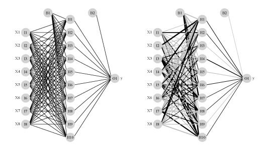
The image on the left is a standard illustration of a neural network model and the image on the right is the same model illustrated as a neural interpretation diagram (default plot). The black lines are positive weights and the grey lines are negative weights. Line thickness is in proportion to magnitude of the weight relative to all others. Each of the eight random variables are shown in the first layer (labelled as X1-X8) and the response variable is shown in the far right layer (labelled as ‘y’). The hidden layer is labelled as H1 through H10, which was specified using the size argument in the nnet function. B1 and B2 are bias layers that apply constant values to the nodes, similar to intercept terms in a regression model.

The function has several arguments that affect the plotting method:

mod.in	model object for input created from nnet function
nid	logical value indicating if neural interpretation diagram is plotted, default T
all.out	logical value indicating if all connections from each response variable are plotted, default T
all.in	logical value indicating if all connections to each input variable are plotted, default T
wts.only	logical value indicating if connections weights are returned rather than a plot, default F
rel.rsc	numeric value indicating maximum width of connection lines, default 5
circle.cex	numeric value indicating size of nodes, passed to cex argument, default 5
node.labs	logical value indicating if text labels are plotted, default T
line.stag	numeric value that specifies distance of connection weights from nodes
cex.val	numeric value indicating size of text labels, default 1
alpha.val	numeric value (0-1) indicating transparency of connections, default 1
circle.col	text value indicating color of nodes, default ‘lightgrey’
pos.col	text value indicating color of positive connection weights, default ‘black’
neg.col	text value indicating color of negative connection weights, default ‘grey’
...	additional arguments passed to generic plot function

Most of the arguments can be tweaked for aesthetics. We’ll illustrate using a neural network model created in the example code for the nnet function:

#example data and code from nnet function examples
ir<-rbind(iris3[,,1],iris3[,,2],iris3[,,3])
targets<-class.ind( c(rep("s", 50), rep("c", 50), rep("v", 50)) )
samp<-c(sample(1:50,25), sample(51:100,25), sample(101:150,25))
ir1<-nnet(ir[samp,], targets[samp,], size = 2, rang = 0.1,decay = 5e-4, maxit = 200)

#plot the model with different default values for the arguments
par(mar=numeric(4),family='serif')
plot.nnet(ir1,pos.col='darkgreen',neg.col='darkblue',alpha.val=0.7,rel.rsc=15,
circle.cex=10,cex=1.4,
	circle.col='brown')

The neural network plotted above shows how we can tweak the arguments based on our preferences. This figure also shows that the function can plot neural networks with multiple response variables (‘c’, ‘s’, and ‘v’ in the iris dataset).

Another useful feature of the function is the ability to get the connection weights from the original nnet object. Admittedly, the weights are an attribute of the original function but they are not nicely arranged. We can get the weight values directly with the plot.nnet function using the wts.only argument.

plot.nnet(ir1,wts.only=T)

$`hidden 1`
[1]  0.2440625  0.5161636  1.9179850 -2.8496175
[5] -1.4606777

$`hidden 2`
[1]   9.222086   6.350143   7.896035 -11.666666
[5]  -8.531172

$`out 1`
[1]  -5.868639 -10.334504  11.879805

$`out 2`
[1] -4.6083813  8.8040909  0.1754799

$`out 3`
[1]   6.2251557  -0.3604812 -12.7215625

The function returns a list with all connections to the hidden layer (hidden 1 through hidden 2) and all connections to the output layer (out1 through out3). The first value in each element of the list is the weight from the bias layer.

The last features of the plot.nnet function we’ll look at are the all.in and all.out arguments. We can use these arguments to plot connections for specific variables of interest. For example, what if we want to examine the weights that are relevant only for sepal width (‘Sepal W.’) and virginica sp. (‘v’)?

plot.nnet(ir1,pos.col='darkgreen',neg.col='darkblue',alpha.val=0.7,rel.rsc=15,
	circle.cex=10,cex=1.4,circle.col='brown',all.in='Sepal W.',all.out='v')

This exercise is relatively trivial for a small neural network model but can be quite useful for a larger model.

Feel free to grab the function from Github (linked above). I encourage suggestions on ways to improve its functionality. I will likely present more quantitative methods of evaluating neural networks in a future blog, so stay tuned!

¹Olden, J.D., Jackson, D.A. 2002. Illuminating the ‘black-box’: a randomization approach for understanding variable contributions in artificial neural networks. Ecological Modelling. 154:135-150.
²Özesmi, S.L., Özesmi, U. 1999. An artificial neural network approach to spatial habitat modeling with interspecific interaction. Ecological Modelling. 116:15-31.