
Collinearity, or excessive correlation among explanatory variables, can complicate or prevent the identification of an optimal set of explanatory variables for a statistical model. For example, forward or backward selection of variables could produce inconsistent results, variance partitioning analyses may be unable to identify unique sources of variation, or parameter estimates may include substantial amounts of uncertainty. The temptation to build an ecological model using all available information (i.e., all variables) is hard to resist. Lots of time and money are exhausted gathering data and supporting information. We also hope to identify every significant variable to more accurately characterize relationships with biological relevance. Analytical limitations related to collinearity require us to think carefully about the variables we choose to model, rather than adopting a naive approach where we blindly use all information to understand complexity. The purpose of this blog is to illustrate use of some techniques to reduce collinearity among explanatory variables using a simulated dataset with a known correlation structure.
A simple approach to identify collinearity among explanatory variables is the use of variance inflation factors (VIF). VIF calculations are straightforward and easily comprehensible; the higher the value, the higher the collinearity. A VIF for a single explanatory variable is obtained using the r-squared value of the regression of that variable against all other explanatory variables:

where the 


Several packages in R provide functions to calculate VIF: vif in package HH, vif in package car, VIF in package fmsb, vif in package faraway, and vif in package VIF. The number of packages that provide VIF functions is surprising given that they all seem to accomplish the same thing. One exception is the function in the VIF package, which can be used to create linear models using VIF-regression. The nuts and bolts of this function are a little unclear since the documentation for the package is sparse. However, what this function does accomplish is something that the others do not: stepwise selection of variables using VIF. Removing individual variables with high VIF values is insufficient in the initial comparison using the full set of explanatory variables. The VIF values will change after each variable is removed. Accordingly, a more thorough implementation of the VIF function is to use a stepwise approach until all VIF values are below a desired threshold. For example, using the full set of explanatory variables, calculate a VIF for each variable, remove the variable with the single highest value, recalculate all VIF values with the new set of variables, remove the variable with the next highest value, and so on, until all values are below the threshold.
In this blog we’ll use a custom function for stepwise variable selection. I’ve created this function because I think it provides a useful example for exploring stepwise VIF analysis. The function is a wrapper for the vif function in fmsb. We’ll start by simulating a dataset with a known correlation structure.
require(MASS)
require(clusterGeneration)

set.seed(2)
num.vars<-15
num.obs<-200
cov.mat<-genPositiveDefMat(num.vars,covMethod="unifcorrmat")$Sigma
rand.vars<-mvrnorm(num.obs,rep(0,num.vars),Sigma=cov.mat)
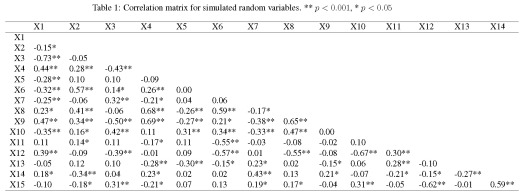
We’ve created fifteen ‘explanatory’ variables with 200 observations each. The mvrnorm function (MASS package) was used to create the data using a covariance matrix from the genPositiveDefMat function (clusterGeneration package). These functions provide a really simple approach to creating data matrices with arbitrary correlation structures. The covariance matrix was chosen from a uniform distribution such that some variables are correlated while some are not. A more thorough explanation about creating correlated data matrices can be found here. The correlation matrix for the random variables should look very similar to the correlation matrix from the actual values (as sample size increases, the correlation matrix approaches cov.mat).
Now we create our response variable as a linear combination of the explanatory variables. First, we create a vector for the parameters describing the relationship of the response variable with the explanatory variables. Then, we use some matrix algebra and a randomly distributed error term to create the response variable. This is the standard form for a linear regression model.
parms<-runif(num.vars,-10,10)
y<-rand.vars %*% matrix(parms) + rnorm(num.obs,sd=20)
We would expect a regression model to indicate each of the fifteen explanatory variables are significantly related to the response variable, since we know the true relationship of y with each of the variables. However, our explanatory variables are correlated. What happens when we create the model?
lm.dat<-data.frame(y,rand.vars)
form.in<-paste('y ~',paste(names(lm.dat)[-1],collapse='+'))
mod1<-lm(form.in,data=lm.dat)
summary(mod1)
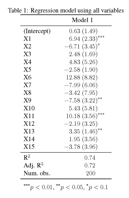
The model shows that only four of the fifteen explanatory variables are significantly related to the response variable (at 
We can try an alternative approach to building the model that accounts for collinearity among the explanatory variables. We can implement the custom VIF function as follows.
vif_func(in_frame=rand.vars,thresh=5,trace=T)

 var vif
 X1  27.7352782054202
 X2  36.8947196546879
 X3  12.5694198086941
 X4  50.7385544899845
 X5  8.35069942629285
 X6  114.685122241139
 X7  67.3415420139211
 X8  153.597012767649
 X9  48.226662808638
 X10 50.7371404106266
 X11 33.9720046917178
 X12 43.2541022358368
 X13 12.0823286959991
 X14 74.6186892947576
 X15 29.8722459010406

removed:  X8 153.597

 var vif
 X1  6.67306561938667
 X2  7.98347501302268
 X3  4.56187657632574
 X4  8.03048468634153
 X5  7.70736760805487
 X6  19.6743072270573
 X7  52.9521670096974
 X9  17.8683960730445
 X10 46.2484642889962
 X11 18.2479446141727
 X12 42.133697798185
 X13 10.8973377491163
 X14 37.9296952803818
 X15 21.5847028917955

removed:  X7 52.95217

 var vif
 X1  6.54376168051204
 X2  7.68236114754164
 X3  4.04873004990332
 X4  5.08958904348524
 X5  2.65685239947949
 X6  9.12685384862522
 X9  2.89940351012031
 X10 4.24712217472346
 X11 4.45202381077724
 X12 12.8835110845825
 X13 1.92759852488083
 X14 6.02382346000219
 X15 8.33332235677386

removed:  X12 12.88351

 var vif
 X1  4.21690743815539
 X2  6.88058249786417
 X3  3.88265091747854
 X4  4.48146995293666
 X5  2.20144300270463
 X6  7.76775127218149
 X9  2.71324446993905
 X10 2.90517847805482
 X11 4.43541888871566
 X13 1.78221291029774
 X14 5.02289299193397
 X15 3.02196822776011

removed:  X6 7.767751

 [1] "X1"  "X2"  "X3"  "X4"  "X5"  "X9"  "X10" "X11" "X13" "X14" "X15"
The function uses three arguments. The first is a matrix or data frame of the explanatory variables, the second is the threshold value to use for retaining variables, and the third is a logical argument indicating if text output is returned as the stepwise selection progresses. The output indicates the VIF values for each variable after each stepwise comparison. The function calculates the VIF values for all explanatory variables, removes the variable with the highest value, and repeats until all VIF values are below the threshold. The final output is a list of variable names with VIF values that fall below the threshold. Now we can create a linear model using explanatory variables with less collinearity.
keep.dat<-vif_func(in_frame=rand.vars,thresh=5,trace=F)
form.in<-paste('y ~',paste(keep.dat,collapse='+'))
mod2<-lm(form.in,data=lm.dat)
summary(mod2)
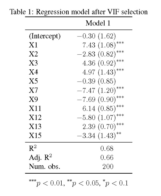
The updated regression model is much improved over the original. We see an increase in the number of variables that are significantly related to the response variable. This increase is directly related to the standard error estimates for the parameters, which look at least 50% smaller than those in the first model. The take home message is that true relationships among variables will be masked if explanatory variables are collinear. This creates problems in model creation which lead to complications in model inference. Taking the extra time to evaluate collinearity is a critical first step to creating more robust ecological models.
Function and example code:
| vif_func<-function(in_frame,thresh=10,trace=T,wts=NULL,...){ | |
| library(fmsb) | |
| if(any(!'data.frame' %in% class(in_frame))) in_frame<-data.frame(in_frame) | |
| if(is.null(wts)) | |
| wts <- rep(1, ncol(in_frame)) | |
| if(!is.null(wts)) | |
| if(length(wts)!=ncol(in_frame)) stop('length of weights must equal number of variables') | |
| if(any(wts < 0)) | |
| stop('weights must be positive') | |
| names(wts) <- names(in_frame) | |
| #get initial vif value for all comparisons of variables | |
| vif_init<-NULL | |
| var_names <- names(in_frame) | |
| for(val in var_names){ | |
| wt <- wts[val] | |
| regressors <- var_names[-which(var_names == val)] | |
| form <- paste(regressors, collapse = '+') | |
| form_in <- formula(paste(val, '~', form)) | |
| vif_init<-rbind(vif_init, c(val, VIF(lm(form_in, data = in_frame, ...)) / wt)) | |
| } | |
| vif_max<-max(as.numeric(vif_init[,2]), na.rm = TRUE) | |
| if(vif_max < thresh){ | |
| if(trace==T){ #print output of each iteration | |
| prmatrix(vif_init,collab=c('var','vif'),rowlab=rep('',nrow(vif_init)),quote=F) | |
| cat('\n') | |
| cat(paste('All variables have VIF < ', thresh,', max VIF ',round(vif_max,2), sep=''),'\n\n') | |
| } | |
| return(var_names) | |
| } | |
| else{ | |
| in_dat<-in_frame | |
| #backwards selection of explanatory variables, stops when all VIF values are below 'thresh' | |
| while(vif_max >= thresh){ | |
| vif_vals<-NULL | |
| var_names <- names(in_dat) | |
| for(val in var_names){ | |
| wt <- wts[val] | |
| regressors <- var_names[-which(var_names == val)] | |
| form <- paste(regressors, collapse = '+') | |
| form_in <- formula(paste(val, '~', form)) | |
| vif_add<- VIF(lm(form_in, data = in_dat, ...)) / wt | |
| vif_vals<-rbind(vif_vals,c(val,vif_add)) | |
| } | |
| max_row<-which(vif_vals[,2] == max(as.numeric(vif_vals[,2]), na.rm = TRUE))[1] | |
| vif_max<-as.numeric(vif_vals[max_row,2]) | |
| if(vif_max<thresh) break | |
| if(trace==T){ #print output of each iteration | |
| prmatrix(vif_vals,collab=c('var','vif'),rowlab=rep('',nrow(vif_vals)),quote=F) | |
| cat('\n') | |
| cat('removed: ',vif_vals[max_row,1],vif_max,'\n\n') | |
| flush.console() | |
| } | |
| in_dat<-in_dat[,!names(in_dat) %in% vif_vals[max_row,1], drop = F] | |
| if(ncol(in_dat)==1) break | |
| } | |
| return(names(in_dat)) | |
| } | |
| } |

Visualizing neural networks from the nnet package – R is my friend
Visualizing neural networks from the nnet package | spider's space
This is a good idea, but why compute VIF = 1/(1-R^2) ? This is a strictly increasing function of R^2, so why not just use R^2 ?
Hi. thanks for the post. I strongly agree your idea. But I am seeking a more efficient way, because calcuating the VIF list for a whole variable set is very time-consuming. I want to ask if there is a way to estimate the variable with high VIF. Thank you
Hi there, you can set the thresh argument to a very high value to keep the algorithm from searching down to the default value of ten. For example:
You should be able to find a maximum value beyond which no variables are removed, though I haven’t tried this.
This is an excellent method for automating feature selection in multivariate linear models. I was able to significantly improve predictability by applying this to the input frame before LM model fitting. Thanks.
Excellent, I’m happy my code was useful!
Thank you for sharing your code, I find it very helpful! I used it to detect collinearity among variables calculated for about 50 objects. The code worked perfectly when the initial number of variable was less than 30. When I tried with more variables (up to 100) for the same 50 objects, I got the following error:
Error in if (vif_max < thresh) { : missing value where TRUE/FALSE needed
I am not expert at using R and I'd like to ask you whether you know the possible cause of this problem. Could it really depend on the number of variables included? Thank you again for the code!!
Hi there, sorry you’re having problems. I can’t reproduce the error using my code:
set.seed(2)
num.vars<-100
num.obs<-200
cov.mat<-genPositiveDefMat(num.vars,covMethod=c("unifcorrmat"))$Sigma
rand.vars<-mvrnorm(num.obs,rep(0,num.vars),Sigma=cov.mat)

#remove collinear variables and recreate lm
vif_func(in_frame=rand.vars,thresh=5,trace=T)
Could you provide an example with your code?
Hi, I did not create the ‘explanatory’ variables (rand.vars), but I used an experimental dataset (X) where each variable represents a certain characteristic of the objects. So I used your code as such on my X matrix, but first I removed all variables with standard deviation equal to zero (same value across all objects). Successively I ran the code on all 100 remaining variables; as I got that error, I only included the first 30 variables and then it worked.
Anyway, as it is working with your 100 ‘random’ variables, the problem must lie in the values of my variables. I will control the dataset better and try again!
Thank you very much for your help and your fast reply!
I’d be curious to hear your solution, as the problem very well could be with my function.
I am receiving the same error message IaIe got: Error in if (vif_max < thresh) { : missing value where TRUE/FALSE needed. I am importing a .csv with 138 explanatory variables, which I don't believe is an issue given your example. There are some variables where every observation is the same. However, I cannot afford to kick out any variables with a standard devation equal to zero like IaIe did. I was wondering if you all found a solution to this by chance? Thanks!
Hi MTV,
Again, I cannot reproduce the error using my code. I used the VIF function with a simulated dataset that contained constant variables (sd = 0) in addition to continuous random variables and did not have a problem:
set.seed(3)
num.vars<-50
num.obs<-200

#continuous random variables, corrrelated
cov.mat<-genPositiveDefMat(num.vars,covMethod=c("unifcorrmat"))$Sigma
rand.vars<-mvrnorm(num.obs,rep(0,num.vars),Sigma=cov.mat)

#constant variables, sd=0
const.vals<-runif(50,-10,10)
const.vals<-matrix(const.vals,nrow=num.obs,ncol=length(const.vals),byrow=T)

#append all variables, randomize column order
rand.vars<-cbind(rand.vars,const.vals)
rand.vars<-rand.vars[,sample(1:ncol(rand.vars))]

#run function
vif_func(in_frame=rand.vars,thresh=5,trace=T)
Is there some way you could post a sample dataset that causes the error? I suspect the problem is not major but I can’t fix it unless I can reproduce the error.
Same error.
Error in if (vif_max < thresh) { : missing value where TRUE/FALSE needed
To debug I put a print commans in ur function vif_func at these positions.:
#get initial vif value for all comparisons of variables
vif_init<-NULL
var_names <- names(in_frame)
for(val in var_names){
regressors <- var_names[-which(var_names == val)]
form <- paste(regressors, collapse = '+')
form_in <- formula(paste(val, '~', form))
vif_init<-rbind(vif_init, c(val, VIF(lm(form_in, data = in_frame, …))))
}
print (vif_init[,2])
vif_max<-max(as.numeric(vif_init[,2]))
print(vif_max)
————————————————————————–
vif_init[,2] had a lot of Inf and NaN values.
vif_max was NaN.
Link to the data set: https://s3.amazonaws.com/fuel-efficiency-modeling/CAX_Train_1.zip
Hi Nara,
Can you please post some code for the dataset you linked to reproduce the error?
Thanks,
Marcus
The error:
Error in if (vif_max < thresh) { : missing value where TRUE/FALSE needed
Will occur if the variables include non-numeric (i.e. nominal variables).
Compliments to the author 🙂
I also had this problem when I tried to use LOO validation and VIF, and the one row that I excluded made one of my regressors to be a fixed column. I did not used factors, only numeric.
Think about a case where a binary column with 100 rows, has a 99 ‘1’ and 1 ‘0’. It will not work.
After I switch some of the ‘1’ to become ‘0’ (not many, just to even it up a bit), it worked.
Hi, this function is very cool.
However, I have a question with your VIF function. According to the fmsb VIF manual, when calculating the VIF for the val in the for loop, the lm function should not be regressed on the whole variable set (your function is
form_in<-formula(paste(val,' ~ .'))
VIF(lm(form_in,data=in_frame,…)
)
But rather should be on all the other variables, excluding the val (
var_names <-names(in_frame)
regressors <- var_names[- which(var_names == val)]
form <- paste(regressors, collapse = '+')
form_in <- formula(paste(val, '~', form)
VIF(lm(form_in,data=in_frame,…)
)
Please let me know if I'm wrong or anything.
Hi there, great blog and Happy New Years!
The function is working fine with my dataset, but when trying to create your sample data, I get an error which is due to the variable/matrix/dataset “y” in your code is only a one column matrix with 200 rows – created in line 74 (y<-rand.vars %*% matrix(parms) + rnorm(num.obs,sd=20))
Is this how it should be? And what is supposed to be %*% doing?
Hope you have time to answer this.
Thanks, M
Sorry for bothering, I just found my mistake: The copy I received had in line 77 only lm.dat<-data.frame(y) and not lm.dat<-data.frame(y,rand.vars)…
So please delete the following entry as well – all is fine
Thanks for reading and I’m glad you like the blog!
Thank you so much for this great tool!
Thanks so much! I was removing explanatory variables with high VIFs all by hand… This has saved me so much time, and it worked in one go, without hassle. Thumbs up.
You’re welcome!
Hi,
Thank you!! Your function worked perfectly with my data
Hi,
I am running your code to try to reduce the number of bioclimatic variables that may be collinear for certain species. Sometimes it seems to work fine, but other times I have infinite values until about the last vif run, leaving usually 1 or 2 variables out of 20, when using a threshold of 10.
Is this right to have these infinite values for so many of the vif runs?
Perhaps my data frame requires transformation first?
Any insight you have would be appreciated
Thanks
Hi there,
An infinite VIF will be returned for two variables that are exactly collinear… variables that are exactly the same or linear transformations of each other. Perhaps check your variables for exact collinearity, using the pairs function or something similar (e.g., ggpairs).
-Marcus
Hi,
Great code, it works well for me, however not well when i have ‘NA’ values. Any idea how i could deal with this?
Thanks
J
Hi J,
I tried running the function with missing data and it works fine for me. The part of the function that handles NA values would be the call to lm, specifically the na.action argument where the default is na.omit. I added an additional argument to the vif_func so you can change this option, though you shouldn’t need to. You could also remove the missing values in your data before using vif_func using na.omit, though you will get a slightly different result since this would remove all rows with incomplete data. Here’s the example I did, note the difference in the final VIF values for the two approaches.
It doesn’t work for me either and when I use na.action=na.omit I receive the following error:
Error in lm.fit(x, y, offset = offset, singular.ok = singular.ok, …) :
0 (non-NA) cases
Hi,
I am running your code and with your data it works fine.
Now I have a data.frame with num and int Variables.
And I am getting the message:
“Error in if (vif_max < thresh) { : missing value where TRUE/FALSE needed"
But there are only numbers, I dont have factors defined or characters.
Do you have any idea, what might be the reason?
The integer values are (0/1)-Results from questions, but I only use the numbers not the translation (no/yes).
Any idea would be very apprechiated
THX
Hi Mark,
Could you provide some example data that causes the problem? This is hard to diagnose if I can’t reproduce the issue.
Thanks,
Marcus
I am getting memory errors that are similar to ones discussed in http://stackoverflow.com/questions/25672974/caught-segfault-error-in-r which I have copied here. Do you have any workaround on this ?
Loading required package: fmsb
*** caught segfault ***
address 0x7f8e32c2d554, cause ‘memory not mapped’
Traceback:
1: terms.formula(formula, data = data)
2: terms(formula, data = data)
3: model.frame.default(formula = form_in, data = in_frame, drop.unused.levels = TRUE)
4: stats::model.frame(formula = form_in, data = in_frame, drop.unused.levels = TRUE)
5: eval(expr, envir, enclos)
6: eval(mf, parent.frame())
7: lm(form_in, data = in_frame, …)
8: summary(X)
9: VIF(lm(form_in, data = in_frame, …))
10: rbind(vif_init, c(val, VIF(lm(form_in, data = in_frame, …))))
Hm, I’ve never seen that error before. I don’t know what the issue is but it may help if the vectors in the function are pre-allocated. I was lazy when I wrote the initial function so the output for each loop simply makes a new copy with each iteration – an inefficient method, expecially in R. Check out this blog for an explanation. I rewrote the vif function with pre-allocated vectors:
#stepwise VIF function with preallocated vectors
vif_func<-function(in_frame,thresh=10,trace=T,...){

  require(fmsb)

  if(class(in_frame) != 'data.frame') in_frame<-data.frame(in_frame)

  #get initial vif value for all comparisons of variables
  vif_init<-vector('list', length = ncol(in_frame))
  names(vif_init) <- names(in_frame)
  var_names <- names(in_frame)

  for(val in var_names){
      regressors <- var_names[-which(var_names == val)]
      form <- paste(regressors, collapse = '+')
      form_in<-formula(paste(val,' ~ .'))
      vif_init[[val]]<-VIF(lm(form_in,data=in_frame,...))
      }
  vif_max<-max(unlist(vif_init))

  if(vif_max < thresh){
    if(trace==T){ #print output of each iteration
        prmatrix(vif_init,collab=c('var','vif'),rowlab=rep('',nrow(vif_init)),quote=F)
        cat('\n')
        cat(paste('All variables have VIF < ', thresh,', max VIF ',round(vif_max,2), sep=''),'\n\n')
        }
    return(names(in_frame))
    }
  else{

    in_dat<-in_frame

    #backwards selection of explanatory variables, stops when all VIF values are below 'thresh'
    while(vif_max >= thresh){

      vif_vals<-vector('list', length = ncol(in_dat))
      names(vif_vals) <- names(in_dat)
      var_names <- names(in_dat)

      for(val in var_names){
        regressors <- var_names[-which(var_names == val)]
        form <- paste(regressors, collapse = '+')
        form_in<-formula(paste(val,' ~ .'))
        vif_add<-VIF(lm(form_in,data=in_dat,...))
        vif_vals[[val]]<-vif_add
        }

      max_row<-which.max(vif_vals)[1]

      vif_max<-vif_vals[max_row]

      if(vif_max<thresh) break

      if(trace==T){ #print output of each iteration
        vif_vals <- do.call('rbind', vif_vals)
        vif_vals
        prmatrix(vif_vals,collab='vif',rowlab=row.names(vif_vals),quote=F)
        cat('\n')
        cat('removed: ', names(vif_max),unlist(vif_max),'\n\n')
        flush.console()
        }

      in_dat<-in_dat[,!names(in_dat) %in% names(vif_max)]

      }

    return(names(in_dat))

    }

  }
Hope that helps.
-Marcus
Thanks for the update. I realized today that the problem might be caused by the large matrix size. I hit the big data ceiling in r. http://www.bytemining.com/2010/05/hitting-the-big-data-ceiling-in-r/
My matrix size was 332 by 47801. I seem to hit the limit at exactly 46341 (46340 works but 46341 doesn’t).
Yep, that was probably the issue. Glad you figured it out though.
Perfect, thank you for sharing!
Hi Prem,
I have the same problem. My function works for 16000 columns but not for 160001. Do you have any suggestion?
Thank you
Hi there, could you post some code (complete with data) that reproduces the example?
Can someone help in analysis of sequential path analysis using grain yield as dependent variable and its component traits as independent variables in R
First of all thanks to share your code! And man.. great ideia to do something like this. I enjoy so much with the method, congratulations for the method!
Hi,
I just wondered if this VIF could help in the feature selection for classification type-models (neural networks) or is just limited to regression type-models?
Thanks,
Alejandro
Hi Alejandro,
The VIF selection could help with fitting neural network models. It will basically tell you which variables are collinear and if they should be removed before creating a model. Collinearity is a problem in most models, not limited to regression. You could try running VIF selection to identify/remove collinear variables prior to creating a neural network. Alternatively, the RSNNS package provides a method for ‘pruning’ a neural network to remove variables that have little influence in the model. I suppose this is similar to variable selection with VIF because it might remove collinear variables, in addition to variables that aren’t related to the response. You could try it both ways to see if you get similar results. There is an example in the help file for the
plotnetfunction that shows how to create and plot a pruned network. Again, you’ll have to download the development version to see this.-Marcus
Hi, this function is very cool.
However, I have a question with your VIF function. According to the fmsb VIF manual, when calculating the VIF for the val in the for loop, the lm function should not be regressed on the whole variable set (your function is
form_in<-formula(paste(val,' ~ .'))
VIF(lm(form_in,data=in_frame,…)
)
But rather should be on all the other variables, excluding the val (
var_names <-names(in_frame)
regressors <- var_names[- which(var_names == val)]
form <- paste(regressors, collapse = '+')
form_in <- formula(paste(val, '~', form)
VIF(lm(form_in,data=in_frame,…)
)
Please let me know if I'm wrong or anything.
Ah, you’re absolutely correct. Thanks for pointing that out. I’ve made changes to the function.
is there corrected code posted here?
Yes, the link above (also here) has been updated.
Hi,
I took the mtcars data set.
To start with, i ran the model without using VIF and got AdjR2 = 0.806.
After that, i used VIF and it eliminated disp, wt, hp, cyl
I ran the model now and i got AdjR2= 0.773.
Here is the code. Not sure why R2 value has dropped after applying VIF. Am i missing something?
#Prior to VIF
summary(lm(mpg~., data=mtcars))
Multiple R-squared: 0.869, Adjusted R-squared: 0.8066
#call the function
vif_func<-function(in_frame,thresh=10,trace=T,…){
…
}
#Use the VIF
require(MASS)
require(clusterGeneration)
require(fmsb)
x <- mtcars[,2:11]
y <- mtcars[,1]
keep.dat <- vif_func(in_frame=x,thresh=5,trace=T)
form.in<-paste('y ~',paste(keep.dat,collapse='+'))
fit<-lm(form.in,data=mtcars)
summary(fit)
Multiple R-squared: 0.8173, Adjusted R-squared: 0.7735
Hi Rajagopalan,
I think a more general problem that might be causing confusion is the type of information desired from a regression model. I would imagine that using more variables could lead to higher R2 values, particularly for collinear variables, as you would be overfitting the model and lowering the residual error. However, your ability to describe relationships between the response variable and each individual explanatory would of course be compromised. I would suggest that removing collinear variables is more important for understanding relationships with the response variable than having large effects on the explained variance. The change is relatively small and both models are not statistically different so I wouldn’t worry too much about minor changes in R2. You might also notice that changing the threshold to 10 raises the R2 value for the second model.
Comparison of the two models shows that they are not statistically different:
library(MASS)

#Prior to VIF
x <- mtcars[,2:11]
y <- mtcars[,1]
form.in<-paste('y ~',paste(names(x),collapse='+'))
fit1 <- lm(form.in, data=mtcars)

# after VIF
keep.dat <- vif_func(in_frame=x,thresh=5,trace=T)
form.in<-paste('y ~',paste(keep.dat,collapse='+'))
fit2 <-lm(form.in,data=mtcars)

# compare
anova(fit1, fit2)
-Marcus
Hi,
I tried this VIF using the above code on the longley dataset.
Case 1. Without VIF, model showed Population, GNP, GNP.deflator not statistically significant by looking at the p-value.
lm(formula = Employed ~ ., data = longley)
Multiple R-squared: 0.9955, Adjusted R-squared: 0.9925
Case 2. I tried the VIF using the above function, It has removed GNP, GNP.deflator and Year. Whereas the Year variable was highly significant without VIF, p-value was 0.003037.
#If VIF is more than 10, multicolinearity is strongly suggested.
VIF(lm(Employed~., data=longley))
VIF is 221 using fmsb package.
keep.dat <- vif_func(in_frame=longley[,-7],thresh=5,trace=T)
form.in<-paste('Employed ~',paste(keep.dat,collapse='+'))
form.in
#Build the model
fit<-lm(form.in,data=longley)
summary(fit)
Multiple R-squared: 0.9696, Adjusted R-squared: 0.962 (using usdm pkg)
Multiple R-squared: 0.9696, Adjusted R-squared: 0.962 (using fmsb pkg)
Questions:
1. Why the VIF removed the Year while doing VIF, since it was highly significant without applying VIF.
2. When there are multi-co linearity between two predictors, should we not remove one and retain the other. Here it seems to be removing both the variables.
Thanks,
Raj
Hi Raj,
Have a look at a pairs plot for the longley dataset:
The VIF function removed all variables except Unemployed, Armed.Foreces, and Population. You’ll notice that the removed variables (Year, GNP.deflator, and GNP) are all collinear with Population. According to the VIF selection criteria, only Population was retained among the four collinear variables.
To answer your first question, year was shown as highly significant in the first model but population was not. After removing year, population is now significant because the two were collinear. This shows that you can get different conclusions from a model if variables are redundant. That’s not to say you can link causal relationships between any of the variables but collinearity can lead to different significance values by including all in the model.
For the second question, both GNP and GNP.deflator were also correlated with Population and, therefore, removed. Again, redundancy among variables lead to different conclusions in the original model.
Hope that helps.
-Marcus
Hi Marcus, first of all thank you very much….this blog is REALLY AMAZING. I just wanted to ask you whether there may be any issue in using this function with 507 variables each of length 127. I expect about 40% of the variables to be highly correlated among each other. I did not get any error message but I didn’t get any output either..I have tried to reduce the sample to 100 variables and results show up after about 1.5 minutes. I have tried 3 time with the full sample and after about 4 hours I still didn’t get any results, so I sarted wondering whether I am doing something wrong. Do you have any idea?
Thank you very much again,
Matteo
Hi Matteo,
I have not tested it with very large datasets but my guess is you’re having problems with sample size. The function runs stepwise regressions for each variable to estimate the VIF. Looking at your sample size vs number of variables, the function would be estimating regressions where the number of observations is much less than the number of variables. This is basically trying to fit regressions with insufficient degrees of freedom to estimate the model parameters. I don’t think you can use the function with this dataset, unless you had a substantially larger sample size.
-Marcus
Thank you so much for this great too!! It works beautifully!
Hi, I see that we can’t use the above function for categorical variables. Please tell me if there is a method to check for collinearity in categorical variables as well.
Hi Srihita,
The variance inflation factor for each variable is from the R2 value of the linear regression of each variable as a function of all other variables. It doesn’t make sense to estimate these values for categorical variables, unless they can be modeled with a GLM with a known distribution family for each categorical variable (e.g., Poisson, Binomial). I don’t think the VIF function in the fmsb package is meant to handle these types of data. I think you would be better off just looking at pairs plots of the explanatory variables to see if there are any patterns worth noting, then deciding for yourself which variables to include. The ‘ggpairs’ plot of GGally can plot both continuous and categorical data in a pairs plot. Hope that helps.
-Marcus
There are number of variable number? Beacuse I try to use with 1555 variables and vif_func() function doesn’t work. Thanks
There shouldn’t be any limit. How many observations do you have for each variable? You should have much more observations than variables.
Hi, did you delete the function code? It’s not showing for me. Thanks
Nope, it’s still there. Can you access it here? https://gist.github.com/fawda123/4717702
It looks like GitHub was for some reason blocked on my side
Thanks a lot, great function
Reblogged this on Topbullets – A Digital Notebook and commented:
A good article for my fellow statistician and analyst
I am an R novice and have been trying to use this VIF function but I don’t understand where to insert the reference to my dataset. It seems like I should reference my data somewhere in this line:
if(class(in_frame) != ‘data.frame’) in_frame<-data.frame(in_frame)
I've tried to do so but to no avail. I'd really appreciate any help! Thanks!
Hi KK,
You need to execute the whole function in your R console so it’s available in your workspace. Then run it as follows, where ‘mydat’ is your data frame:
vif_func(in_frame = mydat, thresh = 5, trace = T)
Make sense?
-Marcus
Hi Marcus,
Thank you so much for the help! I really appreciate it! I understand now that I need to define the function in my console before trying to run it with my own data. I am still having issues unfortunately getting it to run. I deleted my categorical variables (Year, Gender) but still have a few missing data points indicated by “NA” so I tried running the function as such:
vif_func(in_frame=na.omit(mydat),thresh=5,trace=T)
or, vif_func(in_frame=mydat,thresh=5,trace=T, na.action = na.omit)
I am receiving the following error code:
Error in if (vif_max < thresh) { : missing value where TRUE/FALSE needed
I noticed that someone from above had mentioned a similar issue so I've pasted some example data below since I don't have a weblink to it. I'm working with a total of 24 variables with 103 observations each—below is just ten lines of it and it can be copy and pasted into a .csv file.
Thanks so much,
Kelly
ELEV Hindiv tempseas_s ast_s db5_s db10_s da26_s da28_s meantcq_s meantwq_s tmax_s tmin_s summtr_s tempseas_d ast_d db5_d db10_d da26_d da28_d meantcq_d meantwq_d tmax_d tmin_d summtr_d
3179 0.5 27.55823692 11.48371865 0 0 36 28 -1.05599589 14.32508216 35.83333333 -1.055555556 24.05555556 22.06795875 7.77648081 0 0 0 0 -0.114633788 10.32303685 13.83333333 -0.444444444 6.805555556
3183.507324 NA 16.5710059 8.819362132 3.539782624 0 7.094591392 5.318238713 -2.152782654 11.54802056 23.28788846 -3.255080987 15.52471746 15.38058592 7.9642638 2.327662211 0 3.734265092 1.959896681 -1.851159556 10.5828139 20.37700385 -2.8385961 12.0941819
3189.996094 0.6 23.06786912 9.269409443 0.703808286 0 3.205730917 1.937252035 -0.614202422 11.76005838 23.08290828 -0.486503761 15.14160102 22.25090462 8.367404588 0.417613371 0 3.222930368 2.517123526 -0.334985352 10.72734907 19.81862798 -0.304642162 11.60190218
3199.368652 0.714 22.92763456 9.213484216 0.661021737 0 3.261933113 1.982571376 -0.622020829 11.7086418 22.89323658 -0.500526021 14.91921926 21.97331177 8.306003678 0.413745247 0 2.892436823 2.20877642 -0.351044829 10.66439585 19.57419086 -0.329556376 11.38377021
3189.996094 0.5 23.06786912 9.269409443 0.703808286 0 3.205730917 1.937252035 -0.614202422 11.76005838 23.08290828 -0.486503761 15.14160102 22.25090462 8.367404588 0.417613371 0 3.222930368 2.517123526 -0.334985352 10.72734907 19.81862798 -0.304642162 11.60190218
3173 0.625 22.99254293 13.11720422 0 0 1 0 -0.097886394 15.03877879 26.11111111 -0.277777778 16.63888889 24.69805628 11.29338822 0 0 0 0 -0.01913988 13.35951208 18.5 -0.111111111 10.77777778
3180 0.25 22.90767975 9.194963416 0.627538392 0 3.242081002 1.925578578 -0.612764092 11.68070019 22.91207242 -0.496202481 15.02109983 21.94864442 8.30866915 0.435457757 0 2.973313836 2.255109249 -0.353463228 10.66130086 19.71490261 -0.334332996 11.50109273
3166.872 0.625 28.79857797 9.796590048 3.316724236 0 0.354253824 0 -1.44378354 11.18890806 18.19903235 -1.936989189 16.13941111 30.26298849 9.110697753 1.778192918 0 0.759563828 0.345256286 -1.27501582 10.59603464 16.63197951 -1.627447566 13.91707621
NA 0.6 22.79454775 9.057997347 0.886871744 0 1.944901335 0.929482614 -0.606302274 11.61591542 22.79389288 -0.449260626 14.87619339 22.44272413 8.353976923 0.419997312 0 3.550758833 2.803455404 -0.359144136 10.76989337 20.22709752 -0.296479419 11.96385662
Hi KK, try the function now, there was an issue with handling NA values in the data.
As an additional caution, you have many more variables than observations. The VIF values based on the regressions of all predictors against each other are numerically constrained by degrees of freedom. This is why you’re seeing lots of NA values in the output (after you run the updated function).
Hi beckmw
First of all congrats for you excellent work !!!
I am building an R package for my research where I automated many pre-processing steps and would like to use your function inside of it to treat collinearity.
May I use it ? How I would refers to it? Just cite as here https://goo.gl/uxm7w or do you prefer another way ?
Is there another methods to treat collinearity ?
The last question: do you have some recommended reference about collinearity?
Thank you
Hi Elias, you can use any of the code from this blog. It doesn’t need to be cited but I appreciate any recognition. You might also check out this paper here: https://journal.r-project.org/archive/2016-2/imdadullah-aslam-altaf.pdf
It’s a nice overview of methods in R to detect collinearity.
Best,
Marcus
Thank you Marcus I will enjoy it.
One lat doubt: What is the function of “…’ in :
vif_func<-function(in_frame,thresh=10,trace=T,…)
Tks
The ellipsis (…) are used in R functions for optional arguments passed to other functions within the parent function. For this example, the ellipsis can pass additional arguments to the ‘lm’ function, which is used within the VIF function inside of my function. It doesn’t have any importance in this example, I just added it out of habit. Some more info here: http://www.burns-stat.com/the-three-dots-construct-in-r/
Marcus,
You should be seeing an uptick in downloads as your VIF has found its way into the Sherbank Kaggle competition. And it has been helping people scale the tight leader board by degrees. Thanks as well for pointing to pairs and ggpairs.
Could you expand a little bit on variables and observations. I can intuit the problem of too many variables and too few observations, and proper number of observations to variables sounds like a power calculation. So between the two sounds like limitations of inference. Or something.
Chris
Hi Chris, thanks for the heads up. Glad to see this is making the rounds in the competition. It always amazes me how information can spread online… difficult to trace the origin sometimes.
Regarding sample size, of course there will always be a need to have more observations than variables. This is true for any model because it’s an issue with degrees of freedom. Fitting a model to ten variables with ten observations is numerically impossible. The same applies to estimating a VIF value, because the core of all estimates is a simple regression of one variable against the others. I think the issue is compounded for multiple VIF comparisons, as in the above function, given that several regressions are estimated at each step.
In extreme cases, my guess is you’ll see lots of NA values in the estimates as the function progresses and/or the function will not work at all. More generally, it might be worth considering what ‘power’ means in the context of VIF. For most models or tests it means the ability to identify the ‘true’ result given the data. I’m not sure what this means for VIF. The ability to identify the truly collinear variables? Not sure if that flies since it’s not a hypothesis test, at least not as a specific objective.
-Marcus
I do get 50 warnings saying “In summary.lm(X) : essentially perfect fit: summary may be unreliable”. Does anybody know why that is the case? I am still new to R and did not 100% understand the function yet. For example – which variable are we trying to use as a dependent variable & does it change?
Hi Monart,
The function regresses each variable against all others to estimate the VIF values. I think you’re seeing the ‘perfect fit’ warning because some of your variables are exactly the same. These should automatically be removed but you will still see the warnings, which in this case should not affect the results. It would be worth removing perfectly collinear variables before running the function to see if you get a similar result.
-Marcus
Thanks for your reply, that is what I guessed as well 🙂 It does give different results when I remove some variables first. Thanks a lot for this site, it is really helpful!
Thank you sir for this great function. I was wondering about if applying this or the other function to exclude variables with high VIF values is bulletproof approach with respect to predictive power of variables. What I see many strong predictors (tested individually against binary target variable) are being removed in my data set due to high VIF and some weaker pass the VIF test. What is your opinion in general to this issue?
Hi Riki, thanks for your comment. VIF is certainly not bullet-proof. There are several methods for evaluating collinearity, only one of which is VIF. Check out this publication for an overview of others: https://journal.r-project.org/archive/2016/RJ-2016-062/RJ-2016-062.pdf
Generally, I see these tools as more diagnostic of identifying collinearity rather than an explicit ruleset for variable selection. I think it’s up to the analyst to choose variables by hand after considering collinearity with others. This is also complicated by the fact that collinearity considers the relationship of one variable with all others, so individual testing of variables could potentially mask the relationship with others. I guess consider this function as one tool among many that can help with model selection, but it’s not absolute.
Hi there, this is very interesting and helpful, thank you!
I would like to run this function with a specific response variable in my data. How would I update the function call to do this?
Hi Chelsea, the goal of this function is to evaluate collinearity among explanatory variables with the intent that the final, least correlated set will be used to evaluate a response variable. I’m not sure it makes sense to include the response variable within the explanatory variables.
Hi Marcus, thanks for your reply! I don’t think my question was super clear. In the setup for the function, you created a response variable for the model as a linear combination of the explanatory variables using this code:
parms<-runif(num.vars,-10,10)
y<-rand.vars %*% matrix(parms) + rnorm(num.obs,sd=20)
I would like to replace that "created" response variable with a binary outcome variable from my own data (e.g., tobacco use status). I'm new to R (usually a SAS user) and can't quite tell if what I've tried is correctly updating the response variable in the function. I would not include this response variable in the list of potential explanatory variables. Thank you again!
Oh I see now, the function doesn’t use the response variable as input nor is it used internally. Only use the explanatory variables as the first argument in the function. Selection of of the explanatory variables is independent of the response.
Hi Marcus,
Thank you sharing this function. It works like a charm and is very useful. I read through the whole blog which brought further clarity.
Just a quick question: how would you like this code to be cited in a scientific paper/journal article?
Regards,
Irf
Hi Irf, glad you found the code useful. No need to cite the code, but if you want to cite the VIF method you can use use these two:
Zuur, A.F., Ieno, E.N. Smith, G.M. Analysing Ecological Data. Springer, New York.
Montgomery, D.C., Peck, E.A. 1992. Introduction to Linear Regression Analysis. Wiley, New York.
Hi Marcus,
Thank you for sending through the references. I am here with a query. You made it clear in your posts that the response variables are not involved in the process; only predictors are used to compute linear regression models and, finally, the VIF.
So, what I would assume is that in the first step, one predictor variable is taken at a time and is regressed against the rest of the predictors using backward regression. After each regression, the R-squared is calculated which is then input in the VIF formula. Is that correct?
Many thanks
Irf
Yes, that’s the basic process. It’s kind of like leave-one-out cross-validation except here we’re talking about variables not subsets of the data.
Uou! A great function.
Recently the “usdm” package has the “vifstep” and “vifcor” functions.
Thanks for taking the time to do this!
Hello! thanks you so much for this article.
But can we use this code even if explanatory variables are catgorial?
The function relies on repeated linear models where each model tests the regression of one variable against all others. It will not work when it uses a categorical variable as the response.
Hello, this code is amazing! Thanks a lot for sharing this.
I am just wondering whether correlations between dependent and independent variables can be considered, such that among variables showing multicollinearity, the code keeps the independent variable which has the highest correlation with the dependent score.
Thanks, glad you found it useful. But no, that’s not really what this function is intended to do. It’s more of a screening tool before you compare independent/dependent variables. There’s a wealth of information in the stats literature about variable selection methods and screening for collinearity is only one of these tools. The caret package may be a good place to start: https://cran.r-project.org/web/packages/caret/vignettes/caret.html
Hi, thanks so much for sharing your custom function. I tried it on my datasets (more than 20 variables) to do Stepwise multicollinearity analysis and it worked well. Can you tell me how can I acknowledge your work? I plan to share your custom function with my colleagues so it would be better if I put your name and affiliation in the script
Hi Agus, glad you found the function useful. No need for attribution but thanks for asking.
Thank you so much… it really is helpful
Thank you for this code; it is the second time I have returned to it in my research training. I have included your html address in my papers but would also like to know how to reference you in my bibliography – for future users who would like to know where to find your work. Thanks. Emma
Hi Emma, glad you are finding good use for the code. No need for formal attribution, a link to the website is sufficient.
Thank you for your code it works very well with my data!
Thanks for the post ! I am currently using it for an analysis and wanted to know if I can cite the page in my article. Or cite your work in any other way.
Thank you
Hi Anita, glad you were able to use the function. You can use this reference for the VIF method:
Zuur, A.F., Ieno, E.N. Smith, G.M. Analysing Ecological Data. Springer, New York.
Montgomery, D.C., Peck, E.A. 1992. Introduction to Linear Regression Analysis. Wiley, New York.
Hello, I also find this method very helpful. But, I would like to point out that when pairing this method with feature significance (z tests, anovaf) I find that statistically significant features are removed while insignificant features remain after the stepwise process. Is this possible or am I misunderstanding the implementation? Thank you
Hi Daniel, that is entirely possible. I think there should be general agreement among methods, but they often do no produce identical results owing to slight differences in assumptions and how the test are actually calculated.
Hi Marcus,
big thanks for sharing.
I have the same issue as some above: Error in if (vif_max < thresh) { : missing value where TRUE/FALSE needed
I have 80 predictor variables with a high degree of multicollinearity such that an lm() call gives 61 undefined coefficients because of singularities.
I see you have not been able to duplicate the error, so here are my code and data: https://www.dropbox.com/sh/mbjtmklk8njqrs6/AADt3L9iNe0xyRKc-6jMFtusa?dl=0
Cheers,
Andrew.
Hi Andrew,
Thanks for sending me the reprex. I was able to figure out the error. The VIF values are estimated by regressing each predictor on all other predictors and then calculating the VIF as 1 / (1 – R2) for the regression and repeating for the remaining predictors. The algorithm starts by finding the predictor with the highest VIF value, removing it, and repeating the process until all VIF values are below the threshold. In your case, you have a dataset with 80 predictors and 20 observations, so the algorithm is unable to start for the same reason that you cannot fit a regression of all predictors against a single response. You do not have enough observations or degrees of freedom to estimate a VIF value. I would suggest finding another feature selection method. The VIF selection method will not work until you have fewer predictors than observations. Hope that helps.
Marcus
Hi Marcus,
thanks for your reply, have been using the code since with good results. Thanks again for the blog.
I now want to force some variables to remain in the var_names if they are excluded, because inter alia they are from a more reliable source. Could you please comment on the validity of doing this? Neither have I succeeded at doing so – error thrown. Letting the VIF analysis run until through gives me a shortlist of linearly-independent variables. If I then add the vars I need to force to the shortlist, and re-run VIF, the forced variables are again thrown out. Logical, of course. But is there a statistically valid workaround that you know of?
Cheers
Hi Andrew, would it not make sense just to run the function on a data frame of variables that exclude the ones you want to keep? I was thinking I could add an argument to the function that would let you indicate which variables to keep, but it would just run indefinitely if the ones to keep are co-linear. It’s also a larger question of model inference, if you have strong reason to believe that some variables are important and should not be excluded, then there’s no reason to use a “naive” algorithm like the VIF function to remove them automatically. Co-linearity is still an issue, but I would pick variables by hand by calculating all VIF and removing those that are potentially problematic. It’s a greater limitation of any model that relies on correlation/linear association. It will be very difficult to make any inference about causality if predictors are correlated, even if you have strong reason to believe the collinaer predictors are all important.
Hi Marcus
Can you please tell me that is this method applicable to binomial glm too?
Thanks in advance.
Regarding the different variable selection result between regression modeling and random forest – GrindSkills
Hi Marcus, thanks for this helpful script! In line with some of the other questions, is there a way I might give a covariate weighting vector such that in the event of collinear/high-VIF combinations, the lower-weighted of a pair might be retained in each step? I’ve written something like this using correlations (pearson/spearman) but I suspect using VIF would be more robust (I just can’t figure out where I might tweak the script). Thanks for any suggestions! GC
@Giancarlo apologies for the delayed response, this modification might work. There’s an argument for weights where the input is a vector equal in length to the number of variables. You can assign a higher weight to the variable you want to retain (by default, all equal weights).
As in:
Updated function:
vif_func<-function(in_frame,thresh=10,trace=T,wts=NULL,...){

  library(fmsb)

  if(any(!'data.frame' %in% class(in_frame))) in_frame<-data.frame(in_frame)

  if(is.null(wts))
    wts <- rep(1, ncol(in_frame))
  if(!is.null(wts))
    if(length(wts)!=ncol(in_frame)) stop('length of weights must equal number of variables')
  if(any(wts < 0))
    stop('weights must be positive')

  names(wts) <- names(in_frame)

  #get initial vif value for all comparisons of variables
  vif_init<-NULL
  var_names <- names(in_frame)
  for(val in var_names){
    wt <- wts[val]
    regressors <- var_names[-which(var_names == val)]
    form <- paste(regressors, collapse = '+')
    form_in <- formula(paste(val, '~', form))
    vif_init<-rbind(vif_init, c(val, VIF(lm(form_in, data = in_frame, ...)) / wt))
  }
  vif_max<-max(as.numeric(vif_init[,2]), na.rm = TRUE)

  if(vif_max < thresh){
    if(trace==T){ #print output of each iteration
      prmatrix(vif_init,collab=c('var','vif'),rowlab=rep('',nrow(vif_init)),quote=F)
      cat('\n')
      cat(paste('All variables have VIF < ', thresh,', max VIF ',round(vif_max,2), sep=''),'\n\n')
    }
    return(var_names)
  }
  else{

    in_dat<-in_frame

    #backwards selection of explanatory variables, stops when all VIF values are below 'thresh'
    while(vif_max >= thresh){

      vif_vals<-NULL
      var_names <- names(in_dat)

      for(val in var_names){
        wt <- wts[val]
        regressors <- var_names[-which(var_names == val)]
        form <- paste(regressors, collapse = '+')
        form_in <- formula(paste(val, '~', form))
        vif_add<- VIF(lm(form_in, data = in_dat, ...)) / wt
        vif_vals<-rbind(vif_vals,c(val,vif_add))
      }

      max_row<-which(vif_vals[,2] == max(as.numeric(vif_vals[,2]), na.rm = TRUE))[1]

      vif_max<-as.numeric(vif_vals[max_row,2])

      if(vif_max<thresh) break

      if(trace==T){ #print output of each iteration
        prmatrix(vif_vals,collab=c('var','vif'),rowlab=rep('',nrow(vif_vals)),quote=F)
        cat('\n')
        cat('removed: ',vif_vals[max_row,1],vif_max,'\n\n')
        flush.console()
      }

      in_dat<-in_dat[,!names(in_dat) %in% vif_vals[max_row,1], drop = F]

      if(ncol(in_dat)==1) break

    }

    return(names(in_dat))

  }

}